
In part 1 of our series on using spectroscopy to estimate the proportion of secondary structure elements in protein samples, we looked at the technique called circular dichroism. We covered its main theory and applications.
I can already hear you saying: I really enjoyed part 1, and now I want to go and actually perform circular dichroism. Please help me out!
Well, ask, and you shall receive. Read on to learn the circular dichroism sample preparation, and how to interpret and interrogate your data.
Circular Dichroism Sample Preparation: 5 Practical Considerations
Although it’s helpful to know the theory behind your experiments so you can design them judiciously, it’s good to consider their practical and logistical aspects to enable you to optimize your sample and workflow.
Choose a free resource to help you move forward
CHEAT SHEET
Western Blot Cheat Sheet
EBOOK
Free Guide to Protein Expression
To that end, here are five handy pointers on best circular dichroism sample preparation to set up your experiment properly.
1. Purge Your Circular Dichroism Spectrometer with Nitrogen Gas
The UV light to which you expose your sample during a circular dichroism (CD) experiment generates ozone from atmospheric oxygen. When ozone decomposes, it forms oxygen free radicals, which are reactive and extremely good at frying electronic circuitry.
A nitrogen purge provides an inert atmosphere to prevent you from wrecking that expensive spectrometer. So be sure to do this purge before any experiments are performed!
2. Degas Your Sample Buffer
Similarly, oxygen absorbs UV radiation at \(\lambda\) < 200 nm. To get a high-quality CD spectrum that’s not too noisy, we need to remove the dissolved oxygen from your sample buffer.
Most labs are equipped with degassing apparatus. The procedure involves gently stirring your buffer under vacuum for ~30 minutes. To get a rough idea of when your buffer is degassed, stop stirring it and inspect for bubbles on the stirrer bar. If no bubbles are visible, then your buffer is degassed. And, speaking of chemicals that absorb UV…
3. Avoid Sodium Chloride
Chloride anions also readily absorb short-wavelength UV radiation (I like to think of these species as being opaque to UV light) and must be avoided where possible.
This is because it’s the short-wavelength UV radiation that provides us with useful structural information.
Protein samples generally require salts to remain soluble, however. So good alternatives that don’t absorb short-wavelength UV as strongly as chloride are:
- sodium phosphate;
- potassium phosphate;
- potassium fluoride.
If you can’t omit sodium chloride altogether, try to limit its concentration to 50 mM. This is approximately the maximum concentration at which it can be present without completely tarnishing a CD spectrum.
4. Rubbish In, Rubbish Out: Prepare Your Sample Properly
Your sample needs to be >90% pure because contaminant proteins will have their own CD signature and may cause you headaches.
As for sample concentration, that will need practical determination. Start at several mg.ml-1 if possible, then prepare some dilutions and screen them all. Just take some sample buffer to the spectrometer with you and dilute your sample on the fly until you hit the sweet spot.
Ultimately, experience will tell you what the “sweet spot” is. Aim for a spectrum with a decent signal (i.e., one that isn’t a flat line) that doesn’t saturate whatever detector the CD spectrometer is equipped with.
The optimal concentration also depends on the path length of the cuvette. Generally, CD cuvettes are available at 1 and 10 mm. Either way, you’ll likely be working in the \(\mu\)g.ml-1 range.
The 1-mm cuvette option makes CD quite an economical technique with regard to the amount of sample required. And if you don’t intend on heating your sample protein to get a melting curve, you get it back at the end!
5. Care for Your Cuvette
No cheap-o disposable plastic cuvettes for CD, I’m afraid. The cuvettes are made of quartz, which, while not particularly exotic, needs looking after. Check out this handy article on cuvette cleaning for some excellent tips.
Analyzing Your Circular Dichroism Data
You can be the most diligent scientist in the world and adhere to the above circular dichroism practice pointers, but it’s useless if you can’t analyze your data. Here are some pointers to get you going.
Your raw circular dichroism data will be a series of measured ellipticity values for every wavelength in the range specified at the start of the experiment.
Ellipticity takes the units 10-3 degree centimeters squared per decimole (10-3 degrees.cm2.dmol-1). Thankfully, it’s often just written as mDeg or CD. Let’s stick with mDeg for now.
As mentioned already, you can introduce temperature as a variable if you wish to generate a melting curve for your sample.
Plotting ellipticity against wavelength generates a CD spectrum from which the secondary structure composition of your sample can be inferred. The extreme cases of 100% alpha-helix, 100% beta-sheet, and 100% random coil are shown in Figure 1.
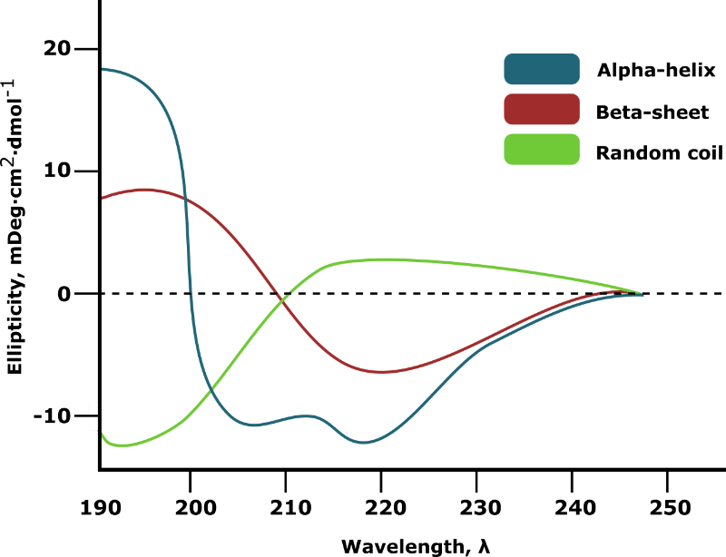
In most cases, your target protein will contain a mixture of secondary structure elements. The relative proportion of each will be virtually impossible to deduce from manual inspection of the spectrum.
Fear not, however, because computational tools can calculate this information (see below for details). However, you’ll need an accurate measure of your sample concentration to get accurate results.
Melting points can be constructed by first collecting CD spectra over a range of temperatures. Then, plot ellipticity at a single wavelength (e.g., mDeg at \(\lambda\) = 210 nm) for every temperature point. You may need to try a few different wavelengths to generate a decent sigmoid.
Apply a sigmoidal fit to the data, and the melting point, Tm, of your sample protein can be calculated from the mid-point of the sigmoid.
Tools for Interrogating Circular Dichroism Data
If you’re lucky, the software that comes with the circular dichroism spectrometer may enable you to graph and interrogate your data. If not, don’t panic, as there are plenty of third-party tools to do this.
The online CD analysis and plotting tool (CAPITO) [1] is reasonably intuitive and can get you started. Otherwise, there are installable programs such as CDtoolX. [2] Both of these tools are free but be sure to ask your resident biophysicist for other options.
From the Vault: My Example Data
I like to show and tell, so check out Figure 2 for some CD data I collected for a troublesome alpha-helical transmembrane protease to bring some reality to all this information.
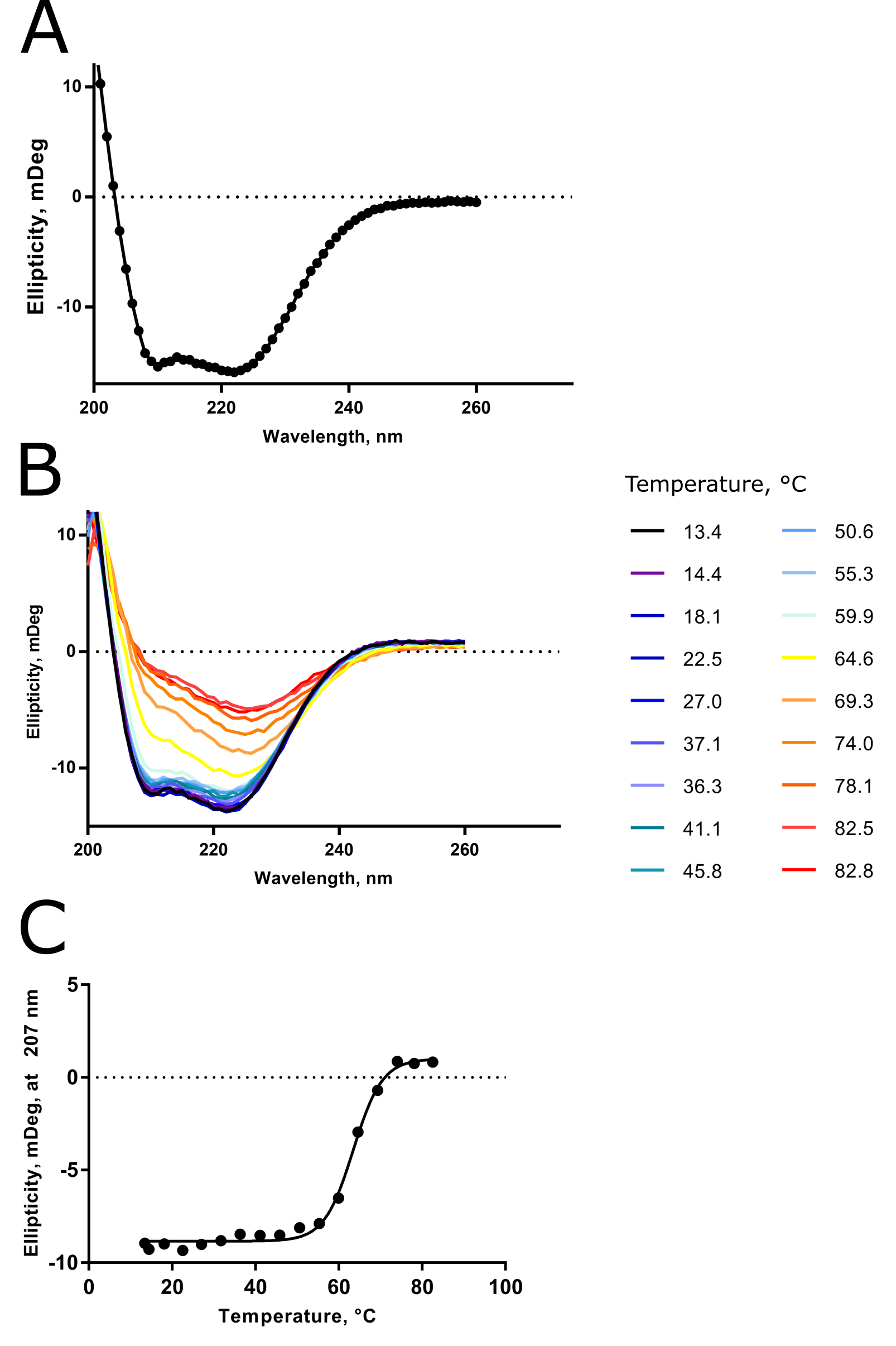
At the time, I had no activity assay, no structure (this is still true), and a funny-looking gel filtration chromatogram due to detergent adsorbing to the column stationary phase. I was happy to learn, via CD, that my sample was folded and relatively thermostable.
In particular, the “double dip” to the room-temperature spectrum at approx \(\lambda\) \(\approx\) 210 and 225 nm told me that my sample was >90% alpha-helical in composition. This result agreed with secondary structure predictions that I had made previously.
The loss of this double dip feature with increasing temperature told me that my protein was unfolding, as you’d expect for thermal denaturation. And spectra taken at ~80°C during the variable-temperature run clearly resemble the 100% random coil scenario presented already in Figure 1.
And finally, from the variable-temperature CD spectra, I was able to determine the Tm of the protease to be ~62°C.
At this point in time, I was used to experiments on membrane proteins failing entirely, and I was glad of some solid data. I wish you gratifying results too.
Have these articles helped you understand circular dichroism practice and circular dichroism theory? Have I missed something important out? Be sure to let us know in the comments section if so.
References
- Christoph W, Peter B, and Matthias G (2013) CAPITO—a web server-based analysis and plotting tool for circular dichroism data. Bioinformatics 29:1750–57
- Andrew J and Miles W (2018) CDtoolX, a downloadable software package for processing and analyses of circular dichroism spectroscopic data. Protein Sci 27:1717–22
You made it to the end—nice work! If you’re the kind of scientist who likes figuring things out without wasting half a day on trial and error, you’ll love our newsletter. Get 3 quick reads a week, packed with hard-won lab wisdom. Join FREE here.


