You’ve found a genetic variant in your data, or you’re planning a study to detect one. This is a practical reference for the six variant classes researchers encounter most often: what each one is, how to detect it, what it does to protein function, and what goes wrong in analysis.
Genetic variants range from a single nucleotide swap to rearrangements spanning whole chromosome arms. Some are harmless. Others drive disease, alter drug metabolism, or determine treatment response.
This page covers SNVs/SNPs, indels, CNVs, translocations, inversions, and repeat expansions, the classes you’ll encounter in most sequencing workflows.
The variant types
Single-nucleotide variants (SNVs) and SNPs
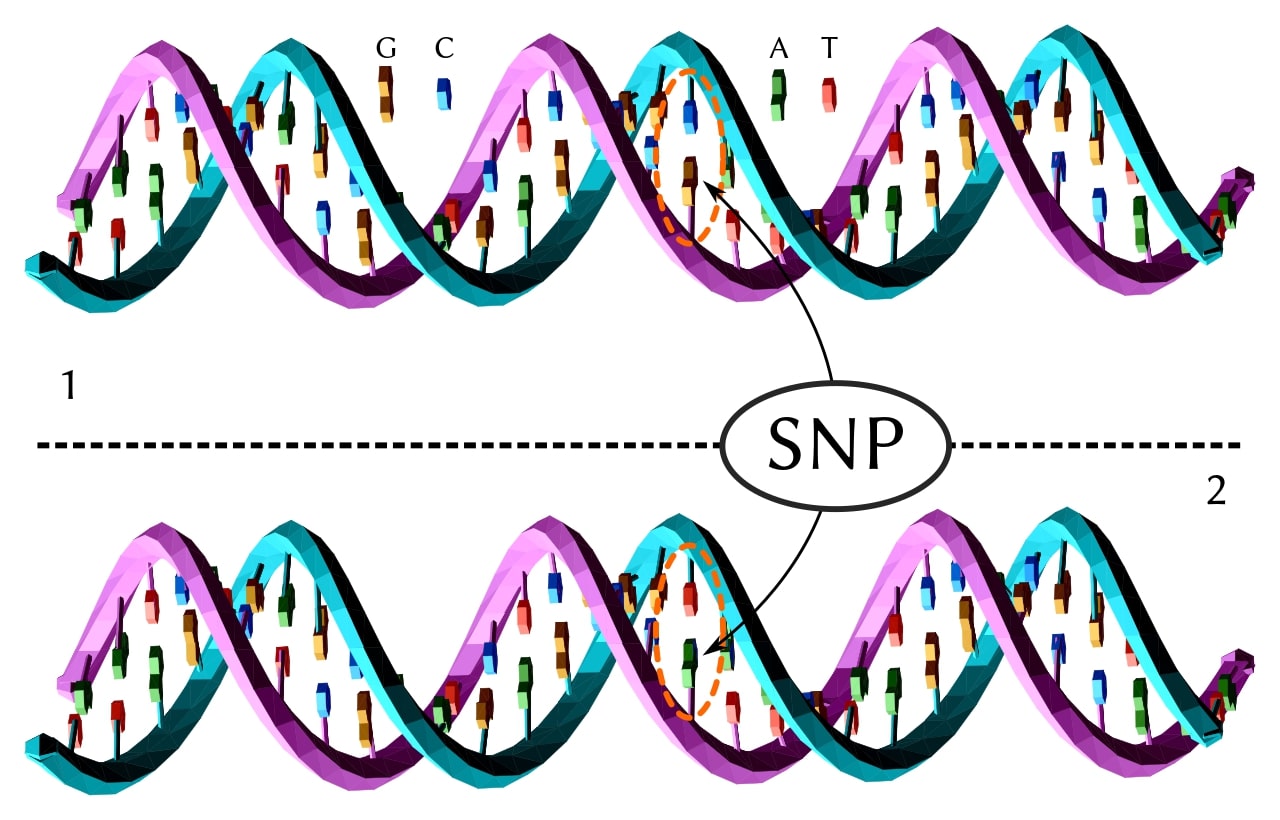
The simplest variant: one nucleotide swapped for another. When an SNV appears in more than about 1% of a population, it’s called a single-nucleotide polymorphism (SNP). A typical human genome carries roughly 4–6 million SNVs relative to the reference, depending on ancestry, reference build, and calling pipeline… African-ancestry genomes tend to carry more, reflecting longer population history. [1]
Most sit in non-coding regions with no known functional effect, but as of a 2018 review, roughly 180 SNPs were associated with breast cancer risk — subsequent GWAS have reported additional loci. [2] Many non-coding variants act by altering expression — see how to go about investigating an expression quantitative trait locus (eQTL).
Choose a free resource to help you move forward
EBOOK
Gene Editing 101
DOWNLOAD
Blood Collection Tube Chart
Insertions and deletions (indels)
Indels insert or delete between 1 and roughly 1,000 base pairs, though definitions vary — some sources place the indel/SV boundary at 50 bp, others higher. Many short-read pipelines treat events ≥50 bp as structural variants. A typical genome carries several hundred thousand indels; exact counts depend heavily on where the boundary is drawn and the depth of sequencing. [3] When the insertion or deletion is not a multiple of three nucleotides, it shifts the reading frame downstream, producing a completely different — and usually nonfunctional — protein.
Cystic fibrosis is the textbook example: a three-base deletion removes a single phenylalanine residue (ΔF508), and that’s enough to cause the disease.
Copy number variants (CNVs)
CNVs are stretches of DNA that are duplicated or deleted relative to a reference genome. In clinical array contexts they typically range from kilobases to megabases, though the boundaries blur — they overlap with large indels at the small end and chromosomal abnormalities at the large end. Despite being fewer in number than SNVs, CNVs can account for more variable base pairs across the genome because of their size.
The human AMY1A gene (salivary amylase) can be present in 2 to 14+ copies per genome — a CNV associated with variation in salivary amylase activity. DiGeorge syndrome most often results from a ~3 Mb deletion on chromosome 22q11.2, making it one of the most common microdeletion syndromes in humans.
Translocations and inversions (chromosomal rearrangements)
Translocations break a DNA segment off one chromosome and attach it to another. Inversions flip a segment 180 degrees within the same chromosome. Whether a rearrangement changes phenotype depends less on its size than on where the breakpoints fall, whether the rearrangement is balanced, and whether any dosage-sensitive genes are disrupted.
Balanced translocations (no genetic material gained or lost) are often clinically silent. Unbalanced translocations are not. The Philadelphia chromosome — a t(9;22) translocation creating the BCR-ABL fusion gene — is found in most cases of chronic myeloid leukaemia.
Repeat expansions
Short DNA sequences — typically 3–6 nucleotides — can be repeated dozens or hundreds of times in a row. When the repeat count exceeds a locus-specific threshold, the result is disease. Huntington’s (CAG repeats in HTT: 36–39 reduced penetrance, 40+ fully penetrant), Fragile X syndrome (CGG repeats >200 in FMR1), and myotonic dystrophy (CTG repeats in DMPK) all follow this pattern, each by a different molecular mechanism.
Repeat expansions often show anticipation: the repeat count tends to grow across generations, making the disease appear earlier and more severely in children than in parents.
Variant type reference
The table below maps what you’re seeing to likely variant classes, showing size range, category, detection methods, a disease example, and functional impact side by side.
Table 1. Common variant classes, detection methods, and functional impact.
| Variant type | Size range | Category | Detection methods | Disease example | Functional impact |
|---|---|---|---|---|---|
| SNV / SNP Single-nucleotide variant / polymorphism | 1 bp | Sequence | SNP arrays, WGS, WES, Sanger sequencing | Breast cancer (~180 risk SNPs as of 2018), sickle cell disease | Missense, nonsense, or silent depending on position. Most are benign; a subset are pathogenic. |
| Indel Insertion / deletion | 1 bp – ~1 kb (boundary definitions vary; many pipelines treat ≥50 bp as SVs) | Sequence | WGS, WES, targeted NGS panels | Cystic fibrosis (ΔF508 — single amino acid deletion) | Can cause frameshift if not a multiple of 3 bp. Often disrupts protein function. |
| CNV Copy number variant | Often kb – Mb in clinical array contexts | Structural | Microarrays (aCGH, SNP arrays), WGS, long-read sequencing | DiGeorge syndrome (22q11.2 deletion), AMY1A gene duplication, Charcot-Marie-Tooth type 1A (PMP22 duplication) | Gene dosage changes. Can amplify or delete functional genes. Although fewer in number than SNVs, CNVs can account for more variable base pairs because of their size. |
| Translocation Chromosomal rearrangement | Kb – whole chromosome arms | Structural | Karyotyping, FISH, WGS, long-read sequencing | CML (BCR-ABL fusion, t(9;22) Philadelphia chromosome) | Balanced: often clinically silent in the carrier, but associated with infertility, recurrent miscarriage, or unbalanced rearrangements in offspring. Unbalanced: gene disruption, fusion genes, developmental defects. |
| Inversion Segment reversal | Kb – Mb | Structural | Long-read sequencing, optical mapping, paired-end WGS | Haemophilia A (intron 22 inversion in F8 gene) | Can disrupt genes at breakpoints. Often missed by short-read sequencing. |
| Repeat expansion Trinucleotide / microsatellite repeat | Repeat unit often 3–6 bp; pathogenic repeat number is locus-specific (tens to hundreds or more) | Sequence / Structural | Repeat-primed PCR, Southern blot, long-read sequencing | Huntington’s (CAG, ≥40 fully penetrant; 36–39 reduced penetrance), Fragile X (CGG, >200 repeats) | Mechanism is locus-specific: toxic polyglutamine protein (Huntington’s), toxic RNA (myotonic dystrophy), methylation silencing (Fragile X), or transcriptional repression (Friedreich’s ataxia). Often shows anticipation. |
Before you start a variant study
- Know your variant size range. SNP arrays are poor for balanced rearrangements, inversions, novel indels, and repeat expansions — but can detect or infer some CNVs. Long-read sequencing catches inversions that short reads cannot. Choosing the wrong platform means missing the variant class that matters most to your study.
- Define your reference genome. Variant calling compares your sequence to a reference. To explore that sequence and its annotations visually, try a genome browser like GeneDig. Using an outdated or inappropriate reference introduces false positives — especially in repetitive regions.
- Plan your sample size. Genome-wide association studies need thousands of samples to detect small-effect variants with statistical confidence. For well-studied genes, targeted panels need far fewer. [4,5]
- Decide WGS vs WES vs targeted panel. Whole-genome sequencing gives the broadest coverage but still has technology-specific blind spots. Whole-exome sequencing covers coding regions only — it misses non-coding regulatory variants. Targeted panels are fast and cheap for known genes, but can’t discover new ones.
- Check whether your variants lie in coding or non-coding regions. If your hypothesis involves regulatory elements, promoters, or epigenetic effects, exome sequencing alone is not enough.
What variants do to proteins
Knowing the variant type gets you to the right detection method. Knowing what the variant does tells you whether it matters. A variant’s functional consequence depends on where it falls in the gene and how it changes the resulting protein.
| Consequence | What happens | Typical impact |
|---|---|---|
| Missense | One amino acid replaced by another | Variable — some are benign, others disrupt protein folding or active sites |
| Nonsense | Amino acid codon changed to a stop codon | Truncated, usually nonfunctional protein |
| Frameshift | Insertion or deletion shifts the reading frame | All downstream amino acids wrong; protein usually nonfunctional |
| Silent / synonymous | Nucleotide changes but amino acid stays the same | Usually benign, though some affect splicing, mRNA stability, translation kinetics, or codon usage |
| Gain of function | Variant gives the protein a new or enhanced activity | Can drive uncontrolled cell growth (oncogenes) |
| Loss of function | Variant reduces or eliminates protein activity | Many recessive loss-of-function disorders require biallelic pathogenic variants, though compound heterozygous, hypomorphic, or splice variants can also fulfil this |
The size of a variant does not predict its impact. A single nucleotide change can cause sickle cell disease, while some multi-megabase CNVs can have surprisingly mild or no apparent phenotypic effects depending on their genomic location and gene content.
Classifying your variant: pathogenic, benign, or uncertain
Once you’ve identified a variant and its functional consequence, the next question is clinical significance. The ACMG/AMP framework sorts variants into five categories. [7] Since 2015, ClinGen’s former Sequence Variant Interpretation working group produced gene- and disease-specific refinements to these criteria. That working group was retired in April 2025; for current recommendations, use ClinGen’s Variant Classification Guidance page alongside the foundational framework.
| Classification | Meaning | What to do |
|---|---|---|
| Pathogenic | Strong evidence the variant causes disease | Report and act on clinically |
| Likely pathogenic | High probability of disease association, not fully confirmed | Report with caveats; follow up |
| Variant of uncertain significance (VUS) | Not enough evidence to classify | Do not use for clinical decisions; flag for reclassification |
| Likely benign | Low probability of disease association | Generally not reported clinically |
| Benign | No evidence of disease association | No action required |
The VUS category is the one that causes the most problems. As sequencing costs fall, VUS results accumulate faster than the evidence needed to reclassify them. Current guidance treats VUS as non-actionable for clinical decisions; periodic reanalysis may be appropriate, particularly when the phenotype remains unexplained. ClinVar entries can also conflict between submitters — use the interpretation from the laboratory most relevant to your phenotype and sequencing context, not just the aggregate label. For a practical walkthrough, BSB’s guide to using dbSNP and ClinVar to classify variants covers the steps.
Detection methods: matching technology to variant type
No single sequencing technology detects every variant type equally well. Choosing the wrong platform is one of the most expensive mistakes in variant analysis. If you’re new to the landscape, BSB’s beginner’s guide to NGS is worth reading before comparing platforms.
| Technology | Best for | Misses |
|---|---|---|
| SNP arrays | Known SNPs, GWAS, population studies | Novel variants, small indels, balanced rearrangements, inversions, repeat expansions, and many SVs outside array probe coverage |
| Targeted NGS panels (hotspot panels covering known oncogenes and tumour suppressor genes, e.g. KRAS, BRAF, EGFR) | Known disease genes, fast clinical screening | Novel genes, non-coding variants, large structural variants |
| Whole-exome sequencing (WES) | Coding variants, rare disease discovery | Non-coding regulatory variants, structural variants, repeat expansions |
| Whole-genome sequencing (WGS) | Broadest single assay for variant discovery, including non-coding and de novo variants; short-read WGS still misses complex SVs, balanced rearrangements, methylation-linked repeat disorders, and some large repeats | Long repeats and complex structural variants (when using short reads) |
| Long-read sequencing (PacBio, Oxford Nanopore) | Structural variants, repeat expansions, inversions, phasing | Raw error profiles differ from short-read sequencing; older long-read chemistries had higher per-base error rates, but PacBio HiFi and improved Oxford Nanopore chemistries have substantially narrowed the gap. Cost per sample still higher than short-read WGS. |
Note: ChIP-seq is sometimes grouped with variant-adjacent methods because it reveals how chromatin state differs between samples — but it characterises epigenetic differences, not DNA sequence variants directly. If your study involves non-coding regulatory effects or histone modifications, ChIP-seq complements sequence-variant data rather than replacing it.
My analysis looks wrong
Variant calling is full of pitfalls. If your results look suspicious, work through these scenarios before trusting or discarding the data. Getting the language right matters too — see homology terminology so you never say the wrong word again.
| Symptom | Most likely cause | Fix |
|---|---|---|
| Hundreds of novel variants in a well-studied gene | Misalignment to reference genome, especially in repetitive regions | Re-align with an updated reference; check mapping quality scores and exclude reads or calls below Q30, as appropriate (Q30 can refer to base quality, mapping quality, or call quality depending on the tool) |
| Known pathogenic variant not detected | Insufficient sequencing depth at that locus, or variant type outside platform’s detection range | Check coverage depth at the specific position; confirm your platform detects that variant class (e.g. short reads miss large inversions) |
| High false-positive rate across the board | Low sequencing depth, PCR duplicates inflating apparent variant frequency, or contaminated sample | Filter PCR duplicates, increase minimum read depth threshold, re-extract DNA if contamination suspected |
| Variant allele frequency stuck at ~50% for every heterozygous call | Normal for germline heterozygous variants; only suspicious if you expected somatic mosaicism | Confirm whether the sample is germline or somatic; somatic variants typically show variable allele frequencies |
| Structural variant calls that don’t validate by PCR | Short-read artefacts at repetitive loci, or split-read caller with high sensitivity but low specificity | Validate with long-read sequencing or FISH; adjust caller specificity settings |
What the textbook doesn’t tell you
Different variant callers disagree with each other. Run the same dataset through GATK, DeepVariant, and Strelka2 and you’ll get overlapping but non-identical variant sets — even with identical inputs. There is no single “correct” caller. For high-confidence results, compare callers where appropriate and validate consequential or novel calls experimentally — orthogonal validation often matters more than simply running more callers. For discovery work, take the union and validate; for clinical or publication use, weigh the sensitivity/specificity tradeoff for your specific context. [6,9]
A VUS today may be pathogenic tomorrow. Variant classification is not static. As population databases grow (gnomAD, ClinVar), variants get reclassified. If you reported a VUS to a patient two years ago, check the current classification — it may have changed.
Repetitive regions are where variant calling goes to die. Roughly 45–50% of the human genome is repetitive sequence, depending on annotation method. Short-read aligners struggle here, and false calls cluster in these regions. If your variant falls in a repeat-rich area, don’t trust it without independent validation.
Population databases have ancestry gaps. Large population databases remain uneven across ancestry groups. [8] Check the ancestry composition and appropriate subpopulation frequencies before filtering — a variant that looks rare in the overall dataset may be common in a specific population, and vice versa.
Common mistakes
| Mistake | How to spot it | How to prevent it |
|---|---|---|
| Using WES to find non-coding regulatory variants | Promising GWAS hits in intergenic regions come up empty in exome data | If your hypothesis involves regulatory elements, use WGS from the start |
| Filtering variants against one population database only | Pathogenic variants in non-European populations flagged as “common” and discarded | Cross-reference multiple databases; check ancestry composition of each |
| Treating all VUS results as benign | Clinically significant variants missed; patients not followed up | Flag VUS for periodic reclassification review; do not dismiss |
| Underpowered sample size for rare variants | Study finds no significant associations despite strong biological rationale | Use power calculations specific to variant frequency and effect size before starting [4,5] |
| Reporting structural variants from short-read data without validation | SV calls don’t reproduce in follow-up experiments | Validate with long-read sequencing, FISH, or PCR across breakpoints |
The decisions that matter most
The logic running through every section here is the same: variant class → detection method → interpretation risk. Get the class wrong and you pick the wrong platform. Pick the wrong platform and you miss the variants that matter. Miss them and your classification work is built on incomplete data.
Three decisions are especially hard to recover from mid-study: calling structural variants from short-read data without a validation plan, filtering against a single population database, and treating VUS results as effectively benign. Underpowered sample size, poor reference genome choice, and batch effects can be just as damaging — but those warrant their own discussion. The three above are the ones most often misread as recoverable when they’re not.
References
- Byrska-Bishop M, et al. (2022) High-coverage whole-genome sequencing of the expanded 1000 Genomes Project cohort including 602 trios. Cell 185(18):3426–3440
- Lilyquist J, Ruddy KJ, Vachon CM, and Couch FJ (2018) Common genetic variation and breast cancer risk — past, present, and future. Cancer Epidemiol Biomarkers Prev 27(4):380–94
- Mullaney JM, et al. (2010) Small insertions and deletions (INDELs) in human genomes. Hum Mol Genet 19(R2):R131–6
- Witte J (2012) Rare genetic variants and treatment response: sample size and analysis issues. Stat Med 31(25):3041–50
- Hong EP and Park JW (2012) Sample size and statistical power calculation in genetic association studies. Genom Inform 10(2):117–22
- Pabinger S, et al. (2014) A survey of tools for variant analysis of next-generation genome sequencing data. Brief Bioinform 15(2):256–78
- Richards S, et al. (2015) Standards and guidelines for the interpretation of sequence variants: a joint consensus recommendation of the ACMG and AMP. Genet Med 17(5):405–24
- Karczewski KJ, et al. (2020) The mutational constraint spectrum from variation in 141,456 humans. Nature 581:434–43
- Wagner J, Olson ND, Harris L, et al. (2023) Variant calling and benchmarking in an era of complete human genome sequencing. Nat Rev Genet 24:464–83
Updated June 2026
You made it to the end—nice work! If you’re the kind of scientist who likes figuring things out without wasting half a day on trial and error, you’ll love our newsletter. Get 3 quick reads a week, packed with hard-won lab wisdom. Join FREE here.