So now you’re convinced that R is the language for you, you’ve downloaded R-Studio (from https://www.rstudio.com/) and opened it, and. . .what the hell do you do now?
Great question!
I always find it easiest to learn by doing something, rather than just by seeing a list of possibilities, so here I’ll walk you through making some fake data, showing it in a boxplot, and doing a t-test to check for differences.
First, when you open RStudio, you should create a new R script, with this button near the top left:
Enjoying this article? Get hard-won lab wisdom like this delivered to your inbox 3x a week.

Join over 65,000 fellow researchers saving time, reducing stress, and seeing their experiments succeed. Unsubscribe anytime.
Next issue goes out tomorrow; don’t miss it.

Now there will be a blank white editor window, which is where we’re going to put the code.
First, enter the following code:
rm(list=ls())
You should always do this at the beginning of any analysis. This line of code removes anything left in the workspace. It is important to clear your workspace before doing something new, so that old leftovers don’t contaminate the new project.
To run the code, highlight it then press Ctrl+Enter. You’ll see it appear in the console, where things get run, after the prompt, looking like this:
> rm(list=ls())
You might as well save the script somewhere now; this should be intuitive enough to not require explaining.
Time to make up some data!
Let’s pretend we did an experiment where we counted the number of chromosomes in cells under two treatments, the control, where we would expect a relatively constant number of chromosomes, and a drug treatment, which increases chromosomal instability and causes aneuploidy (the wrong number of chromosomes). Perhaps the wild type number of chromosomes is 8. If you counted chromosomes in 10 control cells, maybe you counted 8, 9, 10, 6, 7, 8, 10, 8, 8, 8 chromosomes. To enter that into R, you use the c() command, which concatenates things (like numbers) into a row, aka vector. If you try just doing that by putting:
c(8, 9, 10, 6, 7, 8, 10, 8, 8, 8)
into your script and running that line by highlighting and hitting Ctrl+Enter, you’ll see this in the console:
> c(8, 9, 10, 6, 7, 8, 10, 8, 8, 8) [1] 8 9 10 6 7 8 10 8 8 8The blue shows your command and the black, after [1], shows the data. This is great, but you’ll also notice, nothing else happened. Importantly, nothing appeared in the Workspace, which means we didn’t assign this vector of data to any variable. To do that, change the command to look like this:
control_data = c(8, 9, 10, 6, 7, 8, 10, 8, 8, 8)
Now if you run this code, you’ll see the variable “control_data” show up in the Workspace, which should also tell you it is numeric[10], which means it is 10 numbers in a vector. Just like we wanted!
We used the variable name “control_data,” but it doesn’t REALLY matter what you call it. You could have called it “fart” for all RStudio cares. The first caveat is that if you call your variables certain function names, it will screw up those functions. But as long as you make your variables reasonably descriptive, this won’t be an issue. The second caveat is that variable names can’t start with numbers, can’t have spaces in them, and can’t contain special characters.
Let’s make up a drug treatment vector of data and save it as the variable “treatment_data”:
treatment_data = c(8,7,8,13,15,9,8,9,10,8)
Let’s take a look at a boxplot of these two groups of data. Doing that is pretty easy, we just use the boxplot() function. To look at just the control data, use:
boxplot(control_data)
You should see the following in your Files/Plots window:

Perhaps you want to find out the mean and other typical summary stats of your control group. Then you could use the summary() command, like this:
summary(control_data)
which will spit this out in the console:
> summary(control_data) Min. 1st Qu. Median Mean 3rd Qu. Max. 6.00 8.00 8.00 8.20 8.75 10.00Standard deviation is another easy one:
sd(control_data) > sd(control_data) [1] 1.229273To see side-by-side boxplots of the two groups, put a comma between them in the boxplot function:
boxplot(control_data,treatment_data)

Of course, it isn’t very helpful to have unlabeled axes, so let’s label them, using the following parameters within the boxplot function: names, which will be assigned a vector of strings (words within quotes) containing the group labels; ylab, which gives the y-axis label; and xlab, which gives the x-axis label.
How did I find out these options? I typed
?boxplot
Into the console (not the editor window this time) and hit enter, which popped up help in the help tab of the bottom-right window. Doing this (question mark then function name) will bring up help on every function.
As a side note, while you can theoretically enter each line of code into the command window and then hit enter (like we just did to get help), it is much better to write your code in a script, save it constantly, and highlight and run as needed. That way you can easily reproduce what you’ve done later. You’re a scientist: don’t trust your memory.
Here is the command used to make the labeled boxplot, and the plot itself:
boxplot(control_data,treatment_data,names=c(‘control’,’drug’),ylab=’Chromosomes per cell’,xlab=’treatment’)
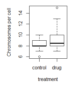
Cool! We have data! So, are the means different? Time to do a t-test! (note: check out this article to learn more about the details of t-tests).
T-tests are also incredibly easy in R, especially the way we’ve got the data set up. We just use the t.test() function, with the first parameter being control_data, and the second parameter being treatment_data:
t.test(control_data,treatment_data)
When run, this outputs:
> t.test(control_data,treatment_data) Welch Two Sample t-test data: control_data and treatment_data t = -1.4524, df = 12.97, p-value = 0.1701 alternative hypothesis: true difference in means is not equal to 0 95 percent confidence interval: -3.2340879 0.6340879 sample estimates: mean of x mean of y 8.2 9.5Leaving most of the interpretation for another day, we can see that p = 0.17, meaning there is a 17% chance that we would see these results if the null hypothesis, that there is no difference between groups, is true. Thus, time to accept the null, collect more data, or get back to the drawing board.
Here is my complete, slightly edited, R script:
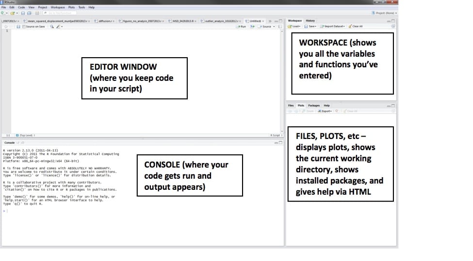
rm(list=ls()) control_data = c(8, 9, 10, 6, 7, 8, 10, 8, 8, 8) treatment_data = c(8,7,8,13,15,9,8,9,10,8) summary(control_data) sd(control_data) summary(treatment_data) sd(treatment_data) boxplot(control_data,treatment_data,names=c(‘control’,’drug’),ylab=’Chromosomes per cell’,xlab=’treatment’) t.test(control_data,treatment_data)Well, that’s it for now. You’ve learned the main places in RStudio, where to keep your code (in a script in the editor window), where your code runs (in the console), where your variables appear (in the workspace), and where plots and help shows up. Furthermore, you’ve learned to enter data, look at it, get some summary stats, and do a t-test!
Stay tuned for more, where we introduce more stats and more detailed R objects, like the awesome data.frame, with which we will eventually make beautiful plots using the ggplot2 package.
You made it to the end—nice work! If you’re the kind of scientist who likes figuring things out without wasting half a day on trial and error, you’ll love our newsletter. Get 3 quick reads a week, packed with hard-won lab wisdom. Join FREE here.