Microsoft Excel can be a really powerful, useful tool for certain kinds of data processing and record keeping, and the chances are you probably don’t even know how to use half of the functions it comes with! That’s OK, personally, I find Excel a bit less user-friendly than Word, but also it’s a programme I never used in school (showing my age here!). I only really started using it when I began my PhD – and even at that, there were many occasions where I would stubbornly sit with a notebook and calculator and work out things the long way rather than spending the time trying to figure out how to do it more efficiently in Excel. Eventually I realised that I needed to bite the bullet and just do a course to refresh some of the basics and also to learn about the some of the advanced functions that I didn’t know existed – hopefully you find a few useful tips or tricks in here.
Back to Basics
Let’s start at the beginning with a quick refresher on formulae and how to use them.
Calculations
One of the main features of Excel is its ability to do calculations, both basic and advanced, to save you the trouble of doing them manually. When you want Excel to do a calculation for you, click on the cell you want your answer in and enter an equals sign to let it know that this cell is to contain a calculation not a name or a single value.
Excel contains numerous pre-programmed functions that you can use in your calculations (we’ll discuss these next time), but first, in order to get your functions to function, you need to make sure you’re referencing your cells correctly.
Cell Referencing
Each cell in Excel has a unique reference ID consisting of the row and column identifiers, e.g. A4 or X345. If you want to incorporate a particular cell into your calculation, you can either manually type this into the formula bar or once you have entered your equals sign into the formula bar you can click on the cell you’re referencing. Now that you’ve entered your cell number, there are two ways to reference a cell in a calculation – absolute referencing and relative referencing.
Let’s start with relative referencing. This is for when you want to use a different value for each calculation; for example, if you have a group of samples that you want to compare with a standard curve. For this scenario, you’re going to create a formula using your first sample, but you’ll want Excel to use the same formula with a different value for each of the other samples. This is really straightforward. All you need to do is type the cell reference as it is, e.g. A6, then when you paste the calculation down your sheet, Excel will move the formula down with it, so the next row will use the same formula but the calculation will use A7 instead of A6. Simple!
Absolute referencing on the other hand is for when you want to use the same value in each calculation, for example the value for your blank that you need to subtract from all other cells. Absolute referencing is also easy; you just need to enter a dollar sign before the row and column number to ensure that the formula uses the same cell for all the calculations, e.g. $A$6. You can do this by either manually typing it into the formula bar or by clicking on the cell and while it is selected, pressing F4.
Your reference can also be a mixture of both absolute and relative referencing, putting a dollar sign ahead of just the row or column number will prevent the formula from moving in that direction, which can be useful if you’re working with slightly trickier calculations.
The Fill Handle
Now that we’ve got referencing down, I want to introduce you to my new friend, the fill handle!

The fill handle is the slightly thicker green corner you see when you select a box. It’s a little bit magical when you figure out how to use it! By left clicking on, and dragging the fill handle down (or up) you will fill all subsequent cells with whatever is in your selected cell – this can be quicker than copying and pasting formulae or values, especially if you’re working with a larger data set! There are other useful properties to the fill handle that I’ll talk about another time, but for now all you need is to know the basics.
Creating a Formula
The key things to remember when creating a formula in Excel are:
- Start with an =
- Always check your brackets are closed at the end!
We’ve already mentioned that all calculations need to start with an = to let Excel know that it is a calculation and not a name, but it’s also important to make sure your formulae are complete; if you’ve used brackets, make sure they’re closed at the end!
Basic calculations are easy to set up;
- Import or type your values in to Excel
- Select the cell that you want your answer in and type =
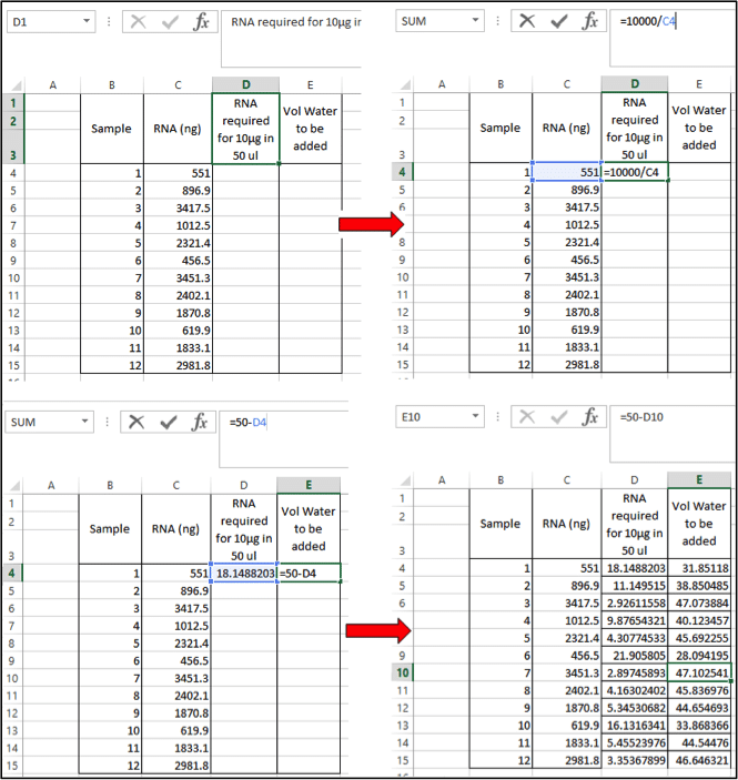
- Figure out what you want Excel to do and write it in the form of an equation. For example: we would like to know the volume of RNA in μl required to yield 10 μg RNA per tube. We then want to dilute to a total volume of 50 μl so that all tubes are at the same concentration and the same volume.
- Equation 1: How many μls of RNA are required? Divide the desired concentration by the concentration in 1 μl
=10000/C4
Equation 2: How much water needs to be added to bring final volume to 50 μl? Subtract the volume of RNA you added from 50
=50-D4 - Copy this formula into your other boxes by dragging the fill handle down
- If you look at the equation for any of your filled in boxes, you will see that the values C4 and D4 have updated themselves to match the row that you are in – this is because we used relative referencing!

Complex Formulae
Now that we’ve seen an easy example, how about something a little more challenging?
Given the values below, you need to normalise all your samples relative to your wild-type control value:

Rather than setting up lots of individual equations, we can use a fairly simple one to do all our calculations at once
- Select your cell and enter =(B3/$A3) – we’re using a mixed reference here because we want the column to remain constant, but the row number to change for each row.
Use the fill handle to drag your equation across and down to fill in your other values and easy peasy! You’ve saved time by not doing a separate calculation for each row.

Tracing Formulae
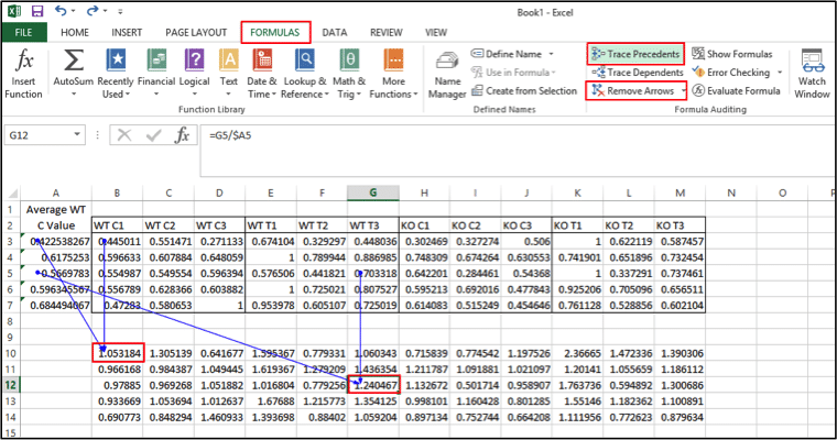
Sometimes mixed referencing can get a little confusing, and at times like that, it’s handy to trace your formula to see what is moving and what is not.
- Click on the formulas tab
- Select the cell you’re unsure of and click “trace precedents” – arrows will appear directing you to the cells that are used in the calculation
- Select as many cells as you want and add precedent for them
- When you’re finished you can simply hit “remove arrows” and they’ll disappear
That’s all for part one. Next time we’ll try using built-in functions and go through a practical example of how you can put all of this together to do calculations in the lab.
What are your useful Excel tricks? Share them below in the comments!
*All screenshots taken from Microsoft Excel 2013 for Windows.


