How to Measure Molecular Weight Using Size-Exclusion Chromatography (SEC)

So, you have a new polymer sample or unknown protein/protein complex and want to know its molecular weight?

A relatively easy way to do this (and purify it at the same time) is size-exclusion chromatography (SEC) which is also known as gel permeation chromatography (GPC).

Interested? Want to learn how to do it and learn a bit more about SEC in the process?

Then stick around as we tell you how to calculate sample molecular weight using size-exclusion chromatography.

How Does Size-Exclusion Chromatography Work?

Let’s go over the basics of SEC before getting into how to use it to measure sample molecular weight.

Size-exclusion chromatography separates analytes by size. How it does so is a little counterintuitive.

In other techniques like gel electrophoresis, we are used to the smaller material moving faster than larger material. But in SEC, higher molecular weight samples elute first.

This is because SEC columns contain beads that have minute pores in them. And these pores are distributed over a range of sizes that are approximately the same dimensions as the intended samples.

As a consequence of this design, smaller samples enter more pores than larger samples as they both pass through the column.

That’s to say, larger samples are “excluded” by the pores.

Add this effect up over a run and what you find is smaller samples enter the pores, spend more time in them, and elute later.

To think of it another way, imagine that these smaller particles “get stuck” in the pores, while large molecules simply pass by them.

This is the mode by which analytes are separated in SEC.

And since the sample size is usually proportional to its molecular weight, the technique can provide the approximate molecular weight of your sample.

The Basic Components of SEC

Let’s look at the SEC components in a bit more detail. Then, with this working understanding, we can learn how to calculate sample molecular weight from a size-exclusion chromatogram.

If you’re in a rush, just check out Figure 1 below.

1. Solvent/Mobile Phase

A wide range of solvents is used in SEC, from non-polar to aqueous, depending on whether you study large chemicals, polymers, or proteins.

Choosing an appropriate solvent for your sample is critical. You need to select a solvent that fully dissolves your studied material. This is because SEC columns are easily blocked by insoluble particulates.

The solvent must also be compatible with the column being used. A common non-polar solvent is tetrahydrofuran (THF), while water can be used as an aqueous solvent.

And if you are analyzing proteins, use a buffer that you know keeps your protein folded, stable, and active.

2. Injector

Some size-exclusion chromatographs have an autosampler with an injector. On the other hand, the ÄKTA systems used to purify proteins often require manual injection using a Luer syringe.

When performing a manual injection, remember to use a blunt-tip needle to avoid damaging the instrument.

Using an autosampler, you can set up a sequence of runs and let them finish while you are working on other tests, drinking coffee, browsing social media, or sleeping.

The important part of using an autosampler is keeping track of the order of your samples. Trust me, you don’t want that confusion after you’ve run a test!

3. Column and Stationary Phase

A size-exclusion column comprises a stationary phase of porous particles all packed together into a column. Like most chromatography columns, it must be kept hydrated at all times.

The porous particles are usually made of an inert polymer such as agarose, cellulose, or dextran.

Size-exclusion columns have working ranges. This range is the approximate upper and lower sample size/molecular weight limits that the column can separate.

That’s to say, to separate your samples, you must have some idea of the molecular weight of your sample(s) to nominate a column with an appropriate working range.

Otherwise, you are stuck finding the correct pore size via trial and error. This might cost you a lot of time and samples.

Other factors to consider when choosing a column include:

1. Ensuring your sample doesn’t stick to the stationary phase.
2. Ensuring the column cannot ionize your sample.
3. Ensuring the column has a sample capacity suited to your needs.

Points 1 and 2 are mainly to avoid blocking the column. Columns are expensive at around $2,000-3,000 at the time of republishing.

4. Pump

The pump pushes the mobile phase and your samples through the column. Pump pressure and flow rate are two important variables in SEC.

Too much pressure and you can damage your sample and the column. Too little pressure and your sample may never elute from the column.

Flow rate is also critical.

A flow rate that is too slow makes the experiment unnecessarily slow, while a flow rate that is too fast can tarnish your results through loss of chromatographic resolution.

This is because SEC is atypical insofar as lower flow rates improve chromatographic resolution, unlike other techniques such as HPLC and GC.

5. Detector and Chromatogram

Numerous types of detectors exist for SEC, including:

1. UV-Vis detectors;
2. Infrared detectors;
3. Refractive index detectors;
4. Density detectors;
5. And small-angle X-ray scattering (SAXS) detectors.

When SEC is combined with refractive index detectors, the technique is termed SEC-MALS (for multi-angle light scattering). It allows for unambiguous determination of sample size and homogeneity and is the gold standard for membrane protein purification.

SEC-SAXS is extremely data rich since SAXS provides a wealth of low-resolution structural information, such as the absolute size of your sample and even an ab initio determination of its shape [1] using program suites such as ATSAS. [2]

But don’t get me wrong, SAXS is not automated and takes expertise and work.

Like those resulting from other analytical techniques, a size-exclusion chromatogram is a graph of peaks corresponding to samples eluting at different points in time.

Using a calibration graph of standards with known molecular weights, the molecular weight of your sample can be calculated.

We’ll demonstrate column calibration in the next section. Before we do that, however, check out the example chromatogram in Figure 2 below to get a feel for how they look.

The Gaussian peak at ~68 mL corresponds to a single purified protein.

Anyway, speaking of column calibration and sample molecular weight…

Measuring Sample Molecular Weight Using Size-Exclusion Chromatography

Let’s get down to what you probably came here for—deducing the molecular of your precious sample.

I’m going to explain this in enough detail that you should be able to run to the lab and have a go yourself after finishing this article!

And I’m going to explain it using an example. Specifically, the calibration of a HiLoad® Superdex 16/600® 200 column with a series of protein standards. This is because I suspect most readers will be using size-exclusion chromatography to purify proteins.

Any substitutions you need to make for your particular application should be obvious, and drop a comment if you have a question.

Calibrate the Column

First, go and get the column equilibrating into filtered and degassed running buffer. We’ll use 20 mM tris, 150 mM NaCl, pH 7.0. This will take a few hours, which gives us time to prepare our standards.

We need to nominate some calibration standards with a molecular weight within the working range of the column. The Superdex 16/600 has a working range of ~10-600 kDa. So we will use the following standards:

• Ferritin (444 kDa);
• Conalbumin (75 KDa);
• Ovalbumin (44 kDa);
• Carbonic anhydrase (29 kDa);
• Ribonuclease A (13.7 kDa);
• Aprotinin (6.5 kDa).

Note that these molecular weights correspond to the specific batches that I used. Please substitute them with the molecular weights supplied with your standards.

Go and prepare them as per Table 1 Below.

Table 1. Size-exclusion chromatography calibration standards recipe.

Make the volume up to 1000 µL by adding 295 µL of the running buffer described above. Then, sterile filter the cocktail and centrifuge it 10,000 x g for 10 minutes to pellet any aggregates.

When the column has equilibrated, inject the cocktail onto the column at a flow rate of ~0.5 mL/min.

After a few hours, you should have a chromatogram like the one below in Figure 3.

It’s wise to collect the peak fractions and run them on SDS-PAGE to confirm their identity.

There are a few additional terms we need to clarify before continuing.

The Void Volume

First, you will notice there is a peak labeled “void”. This corresponds to the void volume.

“What is the void?” I hear you ask.

The void, or void volume, is the volume at which an analyte that doesn’t enter any of the bead pores will elute. In other words, the volume at which any analyte whose molecular mass is above the upper working range limit of the column will elute.

The void volume is a hard upper limit.

Any species too large to enter the bead pores will elute all simultaneously in the void, regardless of their size/molecular weight. Indeed, this must be the case since no separation of these species can occur (because they are too big to enter the pores that yield analyte separation).

You can deduce the void volume for any column by running a whopping great analyte down it. Blue dextran (2000 kDa) is an excellent void volume marker.

The Accessible Volume

Second, you’ll notice that the X-axis of the chromatogram is cut at 120 mL. That’s because this value is the total accessible volume for the column in question.

The accessible volume is simply the total volume of the stationary phase that analytes and solvents can access. Hence the name.

Species whose molecular mass is equal to or below the lower working range limit of the column have access to 100% of the accessible volume. Indeed, that is how the lower working range limit is defined.

In SEC, total accessible volume and column volume are used interchangeably.

Good news!

You don’t need to deduce it like the void volume. It will be provided with the column documentation. Or you can look it up online. Or you can ask an experienced lab member.

Anyway, once we know these two values, we have almost enough information to construct our calibration graph.

Construct a Calibration Graph

There are three parameters, one definition, and one sum that we need to know/understand to construct our calibration graph. The terms are:

1. The void volume (Vo);
2. The accessible volume (Vc);
3. And the analyte retention volume (Ve).

Vo and Vc we have already covered. Ve is simply the volume at which an analyte elutes, taken at the middle of the corresponding peak.

The definition is for the gel phase distribution coefficient, Kav. It’s defined as the fraction of accessible volume available to a single analyte of a given size. We can express that mathematically as:

Kav = (Ve – Vo)/(Vc – Vo)

This is the sum that we need to know.

If you think about it makes sense. Separation begins to occur only after the void volume. So it’s effectively a useless fraction of the total column volume and so must be deducted. Hence the Vc – Vo term.

And of the remaining volume, the Ve – Vo term defines how much stationary phase volume an analyte accesses. As Ve approaches Vc, Kav tends to 1.0 (maximum retention).

Anyway, for all of the analytes in your cocktail of standards, calculate their corresponding Kav values.

Then, plot Kav against the log (to base 10) of their molecular weights. Hey, presto! A linear calibration graph. Our example graph is plotted in Figure 4 below.

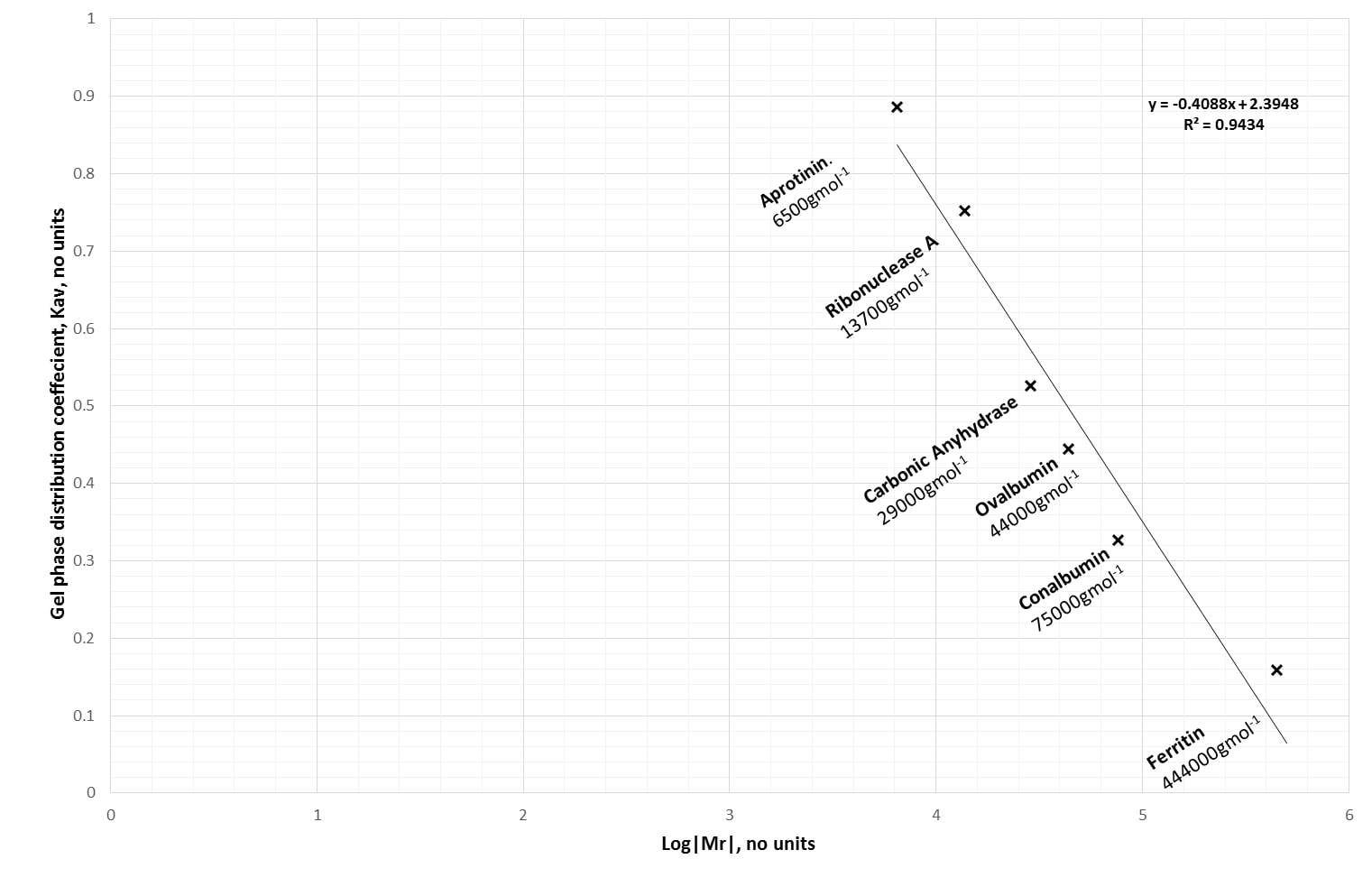
(A pearl of wisdom before continuing—you might want to flip the axes over in your calibration graph. It’s more intuitive to have log|M_r| on the Y-axis.)

Run Your Sample

I’ll leave this bit to you. Try and run it under conditions that you ran the standards under. If you need a more exotic running buffer to stabilize your sample, then fair enough. It’s unlikely to change the validity of the calibration graph, although this is something you might want to check if things go awry.

Do the Maths

Right then, the fiddly bit.

Let’s say we’ve run a sample that eluted at a retention volume of 94.3 mL.

Its Kav would be:

(94.3 – 48.2)/(120 – 48.2)

That comes out at 0.640.

According to our calibration graph in Figure 4, the relationship between Kav and log|M_r| is:

Kav = -0.4088·log|M_r| + 2.3948

Rearranging for log|M_r| gives:

log|M_r| = (Kav – 2.3948)/-0.4088

This comes out at 4.292.

So now all we need to do is reverse the log function by doing the sum:

10^4.292

This gives us a sample molecular weight of 19.6 kDa.

Always Sanity-Check Your Answer

Does this answer make sense?

Well, looking at the calibration chromatogram, 94.3 mL, 19.6 kDa is in the middle of carbonic anhydrase (29 kDa, 80.6 mL) and ribonuclease A (13.7 kDa, 102.1 mL).

So yeah, it does!

Other Sample Characteristics SEC Can Tell You

You can do even more exotic calculations if you like. For example, SEC can provide:

1. The number-average molecular weight (M_n);
2. The weight-average molecular weight (M_w);
3. The z-average molecular weight (M_z);
4. The molecular weight distribution (MWD);
5. And the polydispersity index (PDI).

You’ve probably had enough maths for now, but you can read about these different definitions of molecular weight and how to calculate them here.

A molecular weight distribution typically looks like a bell curve. The left-most end describes high molecular weight molecules, and the right-most end describes low molecular weight ones.

A broad molecular weight distribution peak indicates that there are many sample molecular weights or shapes (see the section below). That is, the sample is polydisperse.

Meanwhile, a sharp molecular weight distribution peak indicates that a sample exhibits a narrow molecular weight range or shape range. That is, the sample is monodisperse.

Monodisperse samples are usually required for experiments such as protein crystallization and enzyme assays.

And if you think about it, besides obtaining the molecular weight of the sample, SEC also provides insight into the different sub-components of a sample, should it have any.

For instance, you can use SEC to interrogate sample oligomerization, sample binding (provided its binding partner is large enough to cause an appreciable shift in retention volume), and stability (e.g., does a special chemical or salt concentration exacerbate polydispersity?)

If your imagination needs a little nudge, see Figure 5 below.

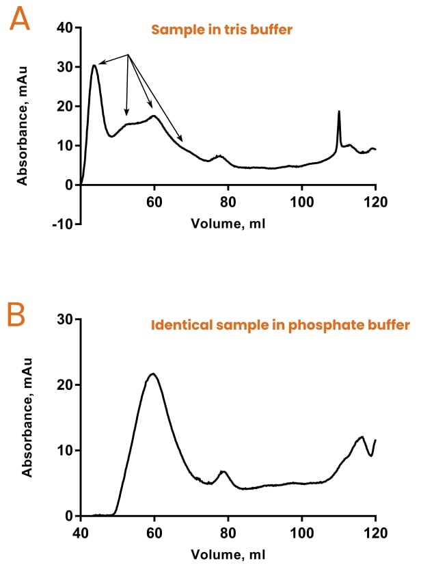
Both chromatograms are for the same protein sample but correspond to different buffer conditions.

The only difference between the two buffers is that one contained 50 mM tris, pH 7.4, and one contained 50 mM potassium phosphate, pH 7.4.

So, according to SEC, tris-based buffers promote polydispersity of this protein as indicated by 4 or 5 unresolved peaks on chromatogram A. This is in contrast to chromatogram B, which demonstrates much greater monodispersity (one main peak).

A Massive Caveat: Sample Size ≠ Molecular Weight

Sample size and molecular weight are not the same and not always proportional.

Lighter molecules can be bigger than heavier ones if they are less compact. Think of rods and fibers.

When I said at the start, “size-exclusion chromatography separates analytes by size,” I meant it literally.

But we are using the size-based SEC chromatogram to infer molecular weight.

That’s why it’s good to couple your SEC experiments with light scattering-based detection methods if possible because they will corroborate or disprove your SEC results.

You’ve been warned!

Molecular Weight and SEC Summarized

We’ve taken a brief look at how size-exclusion chromatography works, a more detailed look at its componentry, illustrated how to use it to calculate the molecular weight of a sample, and warned of its limitations.

So we’ve had a fairly comprehensive look at it! Hopefully, you found this article and its illustrations helpful. Don’t worry if bits of it went over your head—it’s not intuitive and a big topic.

That’s why there’s a comments section!

Does anything need explaining further? Have you had a good experience with SEC/GPC? Use it to let us know.

Originally published July 2016. Revised and updated October 2022.

References

1. Grant TD et al. (2011) Small angle X-ray scattering as a complementary tool for high-throughput structural studies. Biopolymers 95:51730
2. Manalastas-Cantos K et al. (2021) ATSAS 3.0: expanded functionality and new tools for small-angle scattering data analysis. J Appl Cryst 54:343–355