The Basics of NMR Part 3: Multidimensional NMR

Welcome to part three of “The Basics of NMR”, where we dive into multidimensional NMR.

As a brief refresh, this three-part series describes how you can use NMR experiments to characterize your protein of interest.

In part one, we explained some critical points when doing 1D proton NMR and learned how to quickly assess whether a sample protein is folded.

In part two, we learned about spin relaxation rates, such as T1 and T2, etc., and how they can be used to derive the oligomeric state of a sample protein.

In this third and final part, we discuss multidimensional NMR, touch on isotope labeling, and learn about a common 2D NMR experiment that can identify ligand binding sites.

What Is Multidimensional NMR?

It’s a large and complicated subject, so I’ll keep the answer as simple as possible.

In a 1D proton NMR experiment, the spectrum obtained is a plot of intensity vs. chemical shift (in parts per million).

In a 2D NMR experiment, the spectrum obtained has an additional set of chemical shift values. So effectively, the plot is intensity vs. chemical shift vs. chemical shift.

This extra set of chemical shifts (also called frequencies) usually collected ¹³C or ¹⁵N nuclei in addition to the proton (¹H) nuclei.

Plot them all together, and hey presto—a 2D NMR spectrum!

Check out slide 26 of this resource for an example.

What Are the Benefits of Multidimensional NMR?

Simple Answer

Again, the answers are quite high-level and rigorous. But in simple terms, the main benefits are:

1. Improved data resolution.
2. Extra and richer data.

Regarding point 1, this is because the signals from the nuclei are spread over a 2D surface rather than a 1D chart.

Regarding point 2, this is because so-called magnetization transfer can take place between coupled nuclei. This results in cross-peaks that provide extra structural information about the sample and make the assignment of chemical shifts easier.

Detailed Answer

Not satisfied? And wondering why you should bother labeling your protein with NMR-active (¹³C and/or ¹⁵N) isotopes?

Well, instead of simply collecting NMR data on the ~1,000 ¹H nuclei (protons) in your ~100 residue protein, you can now include the ~150 ¹⁵N and ~500 ¹³C nuclei in a multidimensional spectrum to associate the position of each peak with two or more resonance frequencies, thereby vastly enhancing spectral resolution.

This enables the correlation of the chemical shifts of protons with chemical shifts of the ¹³C or ¹⁵N nuclei to which they are attached (although covalent attachment is not necessary).

So, the construction of heteronuclear (i.e., ¹H-¹⁵N, ¹³C-¹⁵N-¹H, etc.) 2D and 3D spectra (via double and triple resonance experiments, respectively) is possible. And this simplifies your NMR data interpretation!

An example of a triple resonance experiment includes ¹H chemical shifts on the x-axis, backbone ¹⁵N chemical shifts on the y-axis, and ¹³C^α chemical shifts on the z-axis.

This is referred to as the “3D HNCA experiment.”

Multidimensional NMR vs. 1D NMR

Using 1D NMR, enormous signal overlap renders it impossible to determine which resonances arise from which nuclei. Typically, signals from 1D NMR can be bunched only into the following groups:

1. Aromatic;
2. Aliphatic;
3. Amide.

Not great resolution, is it?

However, by following ¹H-¹³C-¹⁵N magnetization pathways in your protein, individual resonances can be assigned to their nuclei of origin via multi-dimensional NMR.

See this practical website for an introduction to triple resonance experiments and resonance assignments.

Thus, multidimensional NMR provides a powerful platform to begin dissecting your protein’s structure, function, and dynamics at atomic resolution.

Not many biophysical techniques can offer such information about proteins in solution.

Practical Aspects of Multidimensional NMR

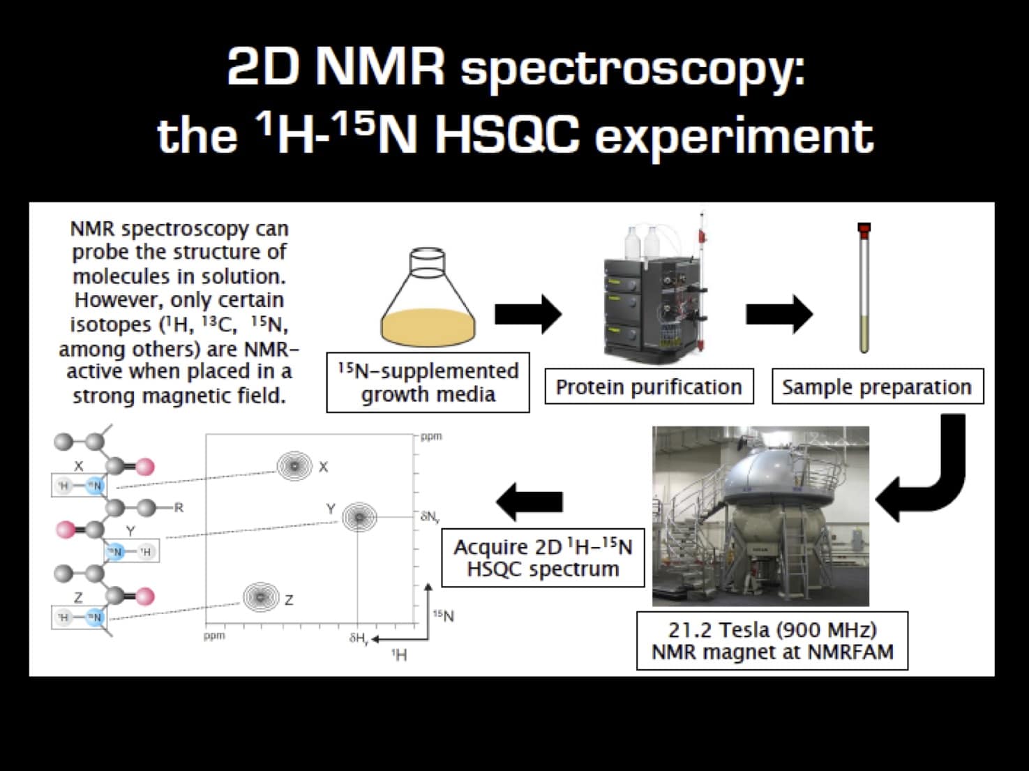
Let’s start with a flowchart outlining the labeling and 2D ¹H-¹⁵N NMR workflow (Figure 1).

Sample Requirements for Multidimensional NMR

In multi-dimensional NMR experiments, which are less sensitive than 1D experiments, you want the concentration of your protein to be as high as possible without aggregation occurring.

Aim for a sample concentration of ~0.3–1.0 mM.

While these concentrations are not necessarily physiologically relevant, it serves to enhance your NMR signals and speed up data acquisition time. If your protein concentration is too low, you will need to collect data for longer.

How to Label a Protein for Multidimensional NMR

If your protein expresses well in E. coli (10s of milligrams per prep), the isotope labeling process is simple.

1. Grow your bugs in M9 Minimal Media and switch out NH₄Cl with ¹⁵NH₄Cl and glucose with ¹³C-labeled glucose.
2. Purify your protein as normal, and boom. Done! 

For 1 L of M9 Minimal Media, you’ll need 1 gram of ¹⁵NH₄Cl and 2 grams of ¹³C-glucose.

All nitrogen atoms will be labeled with ¹⁵N, and all carbon atoms will contain 13C. 

If your protein expresses poorly, you can still label with ¹⁵N and ¹³C, but the process is simply more expensive as you’ll need more isotopically labeled media.

What Can You Do with Multidensional NMR?

Okay, you’ve isotopically labeled your protein. Now what? Well, at the risk of giving you the hard sell, you can:

1. Use the vast suite of 2D and 3D NMR experiments to stretch that mess of overlapped peaks in your 1D ¹H NMR spectrum into multiple dimensions with larger ¹³C or ¹⁵N chemical shift ranges.
2. Pinpoint specific NMR signals to their nuclei of origin within the amino acids of your protein. This process is known as “assigning resonances.”
3. Once a protein’s NMR signals have been assigned to specific nuclei, you can characterize your sample’s structure, dynamics, binding interactions, and functions at atomic resolution.

Pretty powerful, right?

With ¹³C and ¹⁵N labeling, it is possible to assign all resonances for proteins up to ~150 amino acids in length. This is contingent on your sample providing clear NMR spectra.

Larger proteins require ²H (deuterium) labeling, which we will not discuss here.

Characterizing Ligand Binding Sites with Multidimensional NMR

Shall we get our hands dirty with an imaginary case study?

Let’s assume you’ve assigned your protein’s NMR signals to specific residues, and there’s a ligand that binds to your protein. You’re interested in identifying the binding interface upon your protein, but how can you do this?

Using a common 2D NMR experiment called the ¹H-¹⁵N HSQC, which gives one peak for every ¹H attached to a ¹⁵N, you can identify the “fingerprint” of your protein’s backbone and then quickly and easily identify the ligand’s binding interface.

Oh, and two things.

The abbreviation HSCQ stands for Heteronuclear Single-Quantum Coherence.

And ¹H-¹⁵N NMR spectra will provide information on backbone amides and nitrogen-containing side-chains.

Anyway.

Chemical shifts, recorded as the difference between the resonance frequencies of a given nucleus and a reference compound (expressed as parts per million, or ppm), are exquisitely sensitive to nuclei’s chemical and electronic environments.

So, the precise positions of chemical shifts can be accurately followed during NMR experiments.

As such, you can utilize the changes in amide proton (¹H^N) chemical shifts as a proxy to elucidate a ligand-binding site upon your protein. [1]

A Multidimensional NMR Protocol To Identify Ligand-binding Sites

Follow the steps below to identify a ligand-binding site on your isotopically labeled and assigned protein.

1. Collect a 2D ¹H-¹⁵N HSQC spectrum of your protein in its apo state as a reference, which typically takes an hour or two (with uniform sampling) depending on the protein concentration and quality of the spectrum.
2. Titrate in an excess amount of your ligand of interest into a sample of your isotopically labeled protein (at the same concentration in your apo sample) and re-collect the 2D ¹H-¹⁵N HSQC spectrum.
3. Compare the apo and bound state 2D ¹H-¹⁵N HSQC spectra and quantify the changes in ¹H^N chemical shifts, otherwise referred to as “chemical shift perturbation mapping.”
4. Calculate changes in ¹H^N resonances (Δσ_H/N) using the equation below. Δσ_H and Δσ_N are the respective changes in ¹H and ¹⁵N chemical shifts in ppm, and the 1/6 factor scales the ¹⁵N chemical shift axis:

Ask your resident NMR expert for assistance if necessary.

Interpreting the Multidimensional NMR Data

The chemical shift perturbations can be divided into three categories to summarize their effects:

1. Those that experience the largest perturbations or are broadened into noise typically reside at or near the ligand-binding site.
2. Nuclei with mildly perturbed chemical shifts are generally found farther away from the binding interface, experiencing such effects via long-range structural rearrangements induced by ligand binding.
3. Nuclei with no changes in their chemical shifts are (generally) unaffected by the ligand.

You can use PyMOL (or MOLMOL and JMol, etc.) to overlay these chemical shift perturbations onto your protein’s three-dimensional structure and generate a map of your ligand’s binding site onto the structure of your target protein (if known).

I’ve given an example of this process below in Figure 2.

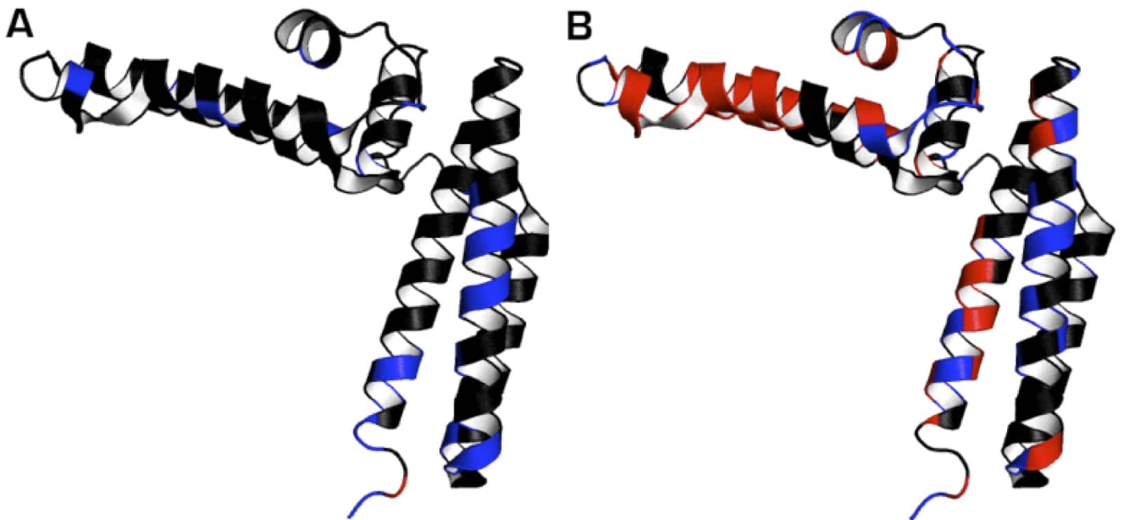
Shown in red are the ¹H^N resonances of ¹⁵N-labeled HscB (PDB: 1fpo) that were broadened out in the presence of an unlabeled ligand. In this case, the ligand was another protein.

In blue are ¹H^N resonances that experienced intermediate chemical shift perturbations (>0.10 ppm).

In black are ¹H^N resonances that were slightly affected (<0.10 ppm) or unaffected by the ligand.

In panels A and B, chemical shift perturbations were mapped onto the structure of HscB in the presence of HscB’s ADP- or ATP-bound chaperone (HscA), respectively.

It’s like magic!

Multidimensional NMR Summarized

We’ve covered a lot of ground there. Answers to all your multidimensional NMR questions. A protocol to determine ligand binding sites. Some example data and fancy images to go along with them!

So, the next time you wish you could specify which residues of your protein are involved in binding to a ligand, why not look toward NMR for assistance? Sure, it involves a bit of legwork. But you get rich data for your effort!

Got anything you want to add? Did I forget to clarify something? Just let me know in the comments section below.

Originally published October 2014. Reviewed and republished June 2022.

Reference

1. Williamson MP (2013) Using chemical shift perturbation to characterise ligand binding. Prog Nucl Magn Reson Spectrosc 73:1–16