Maybe you are sitting in front of your computer wondering whether fluorescence microscopy might be the technique to help you light the bulb on your project. Or you might be in front of a fluorescence microscope, sample in hand, wondering what is actually going on between the sample and the image. Either way—read on!
Fluorescence microscopy is to light microscopy what color TV is to a shadow puppet play. Light microscopy transmits light through a sample to obtain an image based on the absorption or refraction of light in that sample. In contrast, fluorescence microscopy detects light (fluorescence) transmitted back by the sample.
Aided by its wide range of applications with relatively few requirements, fluorescence microscopy has long been an essential tool in biological research. This article will illuminate how fluorescence is generated and detected in the fluorescence microscope. It will also give you an overview of how to use this technique in your research.
How Fluorophores Work: Excitation and Emission!
A fluorophore is the ‘thing’ that generates the fluorescence in your sample. Hang on to your pipette; here comes the physics!
A fluorophore is a molecule in which light of a particular wavelength (a photon) can be absorbed by an electron (See Figure 1). [1] Consequently, this electron jumps to a higher energy level (an orbital further away from the atom nucleus). The electron, and consequently the atom and the molecule containing it, become excited. This process is called excitation.
The excited high-energy state, however, is unstable, and the electron will quickly (i.e., nanoseconds) revert to its ground state. To fit into its ground energy state, the energy previously absorbed must now be dissipated. This is done mostly (but not entirely!) as fluorescence. Due to this “mostly”, the emitted photon has a somewhat longer wavelength (lower energy) than the photon that excited the fluorophore. This process is known as emission.

Fluorescence Spectra and Stokes Shift
A fluorophore can absorb and emit photons with various wavelengths (as excitation and emission spectra, Figure 2). However, all fluorophores have peak wavelengths of excitation and emission depending on their chemical structure. The difference between the excitation and emission wavelengths is termed the Stokes shift. This is what makes fluorescence detectable above the background in a fluorescence microscope.
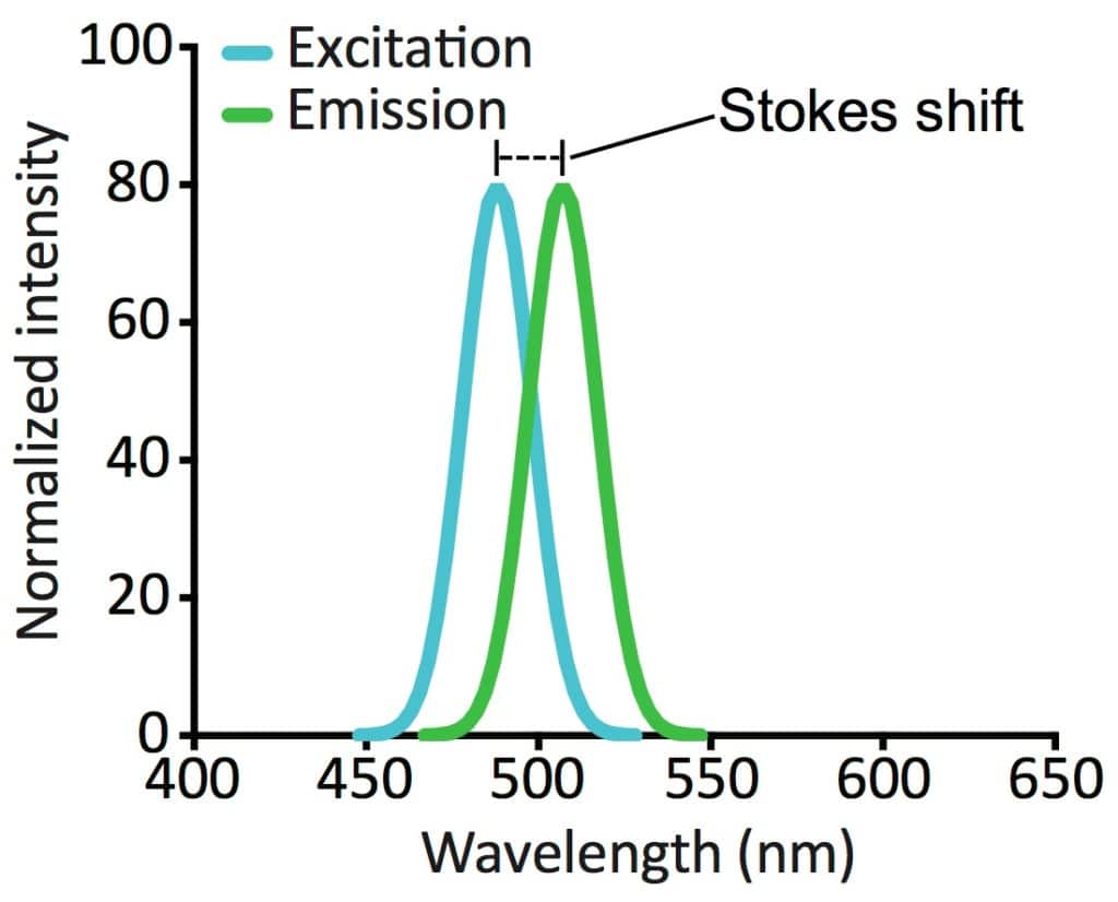
Knowing the excitation and emission spectra of a fluorophore is critical when choosing optimal light sources and filters for your fluorescence microscope, as well as when visualizing more than one fluorophore in a sample.
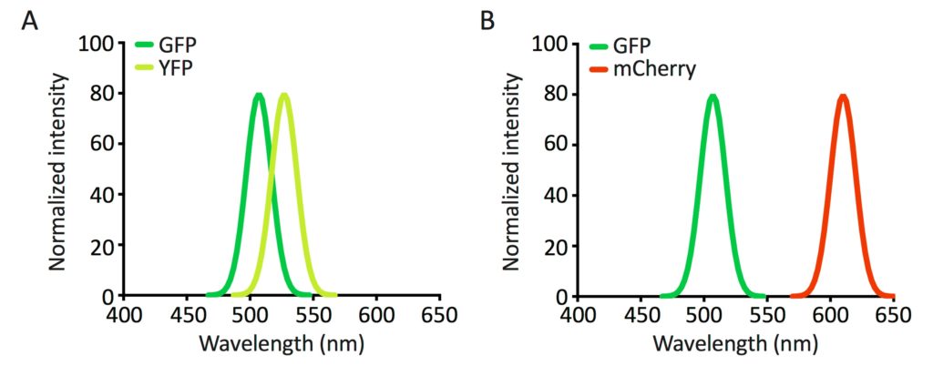
If the emission spectra of the two fluorophores overlap significantly (Figure 3A), the signal of one fluorophore will bleed through in the detection of the other. Therefore, if you want to detect the signal of two fluorophores, choose these so that their emission spectra do not overlap (Figure 3B).
Visualizing Fixed Samples with Immunofluorescence
Fluorophores come in all shapes, sizes, and colors. They can visualize many biological molecules, structures, and phenomena—including everything from ions to whole organisms, live or fixated.
Short of your sample being naturally autofluorescent (e.g., chlorophylls in plant tissue), immunostaining of fixated samples probably allows the easiest and most tailored approach to fluorescence microscopy of your sample. The fluorophore, in this case, is a fluorescent molecule conjugated with an antibody. Virtually all the colors of the rainbow are available—just take your pick.
Usually, immunostaining is performed as a two-step labeling approach:
- A primary antibody detects the antigen.
- A fluorophore-conjugated secondary antibody subsequently detects the resulting immune complex.
In essence, if there is a primary antibody available to detect your nucleic acid, protein, or post-translational modification of interest, you can visualize it by immunostaining followed by fluorescence microscopy—in cells and tissue samples.
What About Live Cell Fluorescence Staining?
Since fixation effectively kills cells, immunostaining naturally falls short in visualizing live samples.
To circumvent this issue, fluorescent proteins (FPs) are used as the source of fluorophores in live cell staining.
Since the discovery of the Green Fluorescent Protein (GFP) in the jellyfish Aequorea Victoria, [2] a whole suite of FPs has been made available through genetic engineering. These can be genetically encoded as fusions with your protein(s) of interest and visualized in samples of single cells to whole organisms. For those of you who are hungry for details, Chudakov et al. provide a comprehensive review of the history, development, considerations, and usages of FPs. [3]
FP-tagging can help track the localization, abundance, and changes within your tagged protein(s) over time and/or in response to given treatments. Furthermore, tagging organelle-specific proteins is one way to mark these subcellular structures.
Organelle-specific Dyes
Alternatively, subcellular compartments can be labeled by membrane-permeable, organelle-specific dyes. Examples are MitoTracker™ (Invitrogen™) and LysoTracker™ (Invitrogen™) for mitochondria and lysosomes, respectively.
Another class of widely used dyes is fluorescent DNA intercalating agents. DAPI (4′,6-diamidino-2-phenylindole) and Hoechst are widely used dyes used to stain and visualize DNA in both live and fixed samples.
Specialized Fluorescent Dyes
Fluorescent dyes that can monitor changes in ion concentration, voltage, and pH are also available. These studies rely on fluorescently labeled chelators whose spectral properties shift with the concentration of a given ion (e.g., fura-2 or indo-1 for calcium ions). You can read information and links to further descriptions of different types of fluorophores here.
Ok, so your sample is ready—a virtual microscopic disco. Just stick it in your fluorescence microscope and wait for the magic to happen. But what is this big box, and what does it actually do? How does it capture your instantly publication-worthy images?
Inside a Fluorescence Microscope: How it Works
Beware! Now the terminology will get somewhat technical as we peek inside the panels to trace the path from the light source to the image through the key components of a fluorescence microscope (Figure 4).[1]

Our journey starts at the light source. In a widefield fluorescence microscope, this is similar to a normal light bulb emitting white light. However, to efficiently excite the fluorophore, only the light corresponding to the peak excitation wavelength must reach the sample. This and more are accomplished in the filter cube.
The Filter Cube, Close Up
The filter cube consists of an excitation filter, a dichroic mirror, and an emission filter. The first thing the white light encounters is the excitation filter. This filter only allows light of the appropriate excitation wavelength to pass through.
Thus filtered, the excitatory light hits the dichroic mirror. This is a special kind of mirror/filter that sits at a 45° angle relative to both the excitatory light and the sample. The dichroic mirror is the key to separating the excitatory light from that emitted by the fluorophore.
Based on its filtering ability, it reflects the excitatory light towards the sample but allows light of a longer wavelength (i.e., the fluorescence) to pass straight through.
En route to the sample, the excitatory light now passes through the objective. The objective magnifies the image but also focuses the excitatory light on the sample. Thus excited, the fluorophore in the sample emits fluorescence. The fluorescence also passes through the objective on its way back toward the filter cube.
Once inside the filter cube, the longer wavelength fluorescence passes through the dichroic mirror and encounters the emission filter. This filter is a so-called band-pass filter, meaning that it only allows light of a certain wavelength interval to pass (i.e., light in the interval where the emission intensity for the fluorophore is at its highest). Light of this wavelength passes through the filter, while any other contaminating or background fluorescence is filtered out.
Finally, the fluorescence hits a prism, which reflects the light toward the eyepiece of the microscope or a camera (or both) to capture high-resolution images of the sample. Et Voilà! Your fluorescent sample has been recorded for posterity.
Applications for Fluorescence Microscopy
There are several things to bear in mind when acquiring images of your sample using a fluorescence microscope. Considerations include balancing brightness, contrast, and photobleaching, [1,3] while key possibilities include the detection of more than one fluorophore in the same sample, generation of 3D images, and following the fluorophore(s) in a sample over time.
Detecting Multiple Fluorophores
This is accomplished by having excitation and emission filters mounted on filter wheels. These can rotate and change both filters synchronously to detect the signal from several fluorophores with high precision and in quick succession. This enables co-localization and interaction studies and allows you to capture rapid dynamic changes in your sample.
3D Visualization of Cellular Structures
Many fluorescence microscopes offer the opportunity of acquiring images of the sample in optical sections (or Z-stacks). This enables 3D visualization of cellular structures and is greatly aided by the advent of confocal microscopes.
The widefield fluorescence microscope captures images in the focal plane, but it also detects some out-of-focus light in the sample resulting in a blurry picture.
The confocal microscope avoids this by laser-mediated illumination of a single spot at a time. This facilitates capturing only the fluorescence from this spot and then scanning across the sample to generate the image.
Live-Cell Microscopy and Time-lapse
Finally, live-cell microscopy becomes very powerful when introducing the fourth dimension: by conducting a fluorescence time-lapse experiment. Time-lapse experiments acquire many images over time instead of brief snap-shots of the cellular environment.
You can use time-lapse fluorescence microscopy to reveal dynamic changes to the cellular milieu with treatment, cell cycle stage, etc., effectively generating your own (potentially multi-colored and 3D) movie with your cells as the stars!
Fluorescence Microscopy Summarized
We’ve explained the principles of how fluorescent molecules emit light, how fluorescent microscopes work, and the different applications of fluorescence microscopy. Got any other uses, or information? Leave a comment below.
If you are not already the proud owner of a fluorescence microscope and are itching to spend a good deal of this year’s research budget on one, check out Bitesize Bio’s guide to buying a fluorescence microscope, and the 2012 review by Eliceiri et al. on software available for acquiring, visualizing and analyzing the images produced by your new magic box. [4] Happy imaging!
Want a stunning, colorful poster that summarizes all the critical fluorescent protein properties like absorption and emission spectra, relative brightness, and quantum yield? Download Bitesize Bio’s ultimate guide to fluorescent proteins poster and stick it up in your lab!
References
- Lichtman JW & Conchello JA (2005) Fluorescence microscopy. Nat Methods 2(12):910-919.
- Shimomura O, Johnson FH, & Saiga Y (1962) Extraction, purification and properties of aequorin, a bioluminescent protein from the luminous hydromedusan, Aequorea. J Cell Comp Physiol 59:223-239.
- Chudakov DM, Matz MV, Lukyanov S, & Lukyanov KA (2010) Fluorescent proteins and their applications in imaging living cells and tissues. Physiol Rev 90(3):1103-1163.
- Eliceiri KW, et al. (2012) Biological imaging software tools. Nat Methods 9(7):697-710.
Figures (generated by the author unless otherwise stated).
Originally published April 2017. Reviewed and updated December 2022.