An Exploration of the Sigmoidal Curve – Math for the Rest of Us

ELISA (Enzyme-Linked Immunosorbent Assay) is the heartbeat of many labs in the research world, owing to its simplicity and its ability to answer a very basic question: how much of protein/peptide/antibody is in my sample?  More specifically, it can be used to answer such questions as:

• How much IgG is in the serum after I give a mouse this vaccination?
• Does IgA spike in the breast-milk during this infection?
• Can I detect a change in albumin levels in stool samples of my heart disease monkey model?

The questions go on and on. If you want to learn more about ELISAs, we have a slew of articles you can check out here, here, and here.  The simplicity of the assay has a tendency to make us lazy, though, and perhaps not appreciate the core of the assay – the standard curve.  Without it, our assay turns into a binary “yes/no” test.  With it, we can dive into the minutia of biological responses.  So, what makes the standard curve so powerful?  Let’s talk about it in the context of ELISAs.

Standard Curves – The Eyeball Test

In its simplest form, the standard curve is a series of positive controls where the amount of target protein is known.  For example, if you are performing an ELISA against human IgG, your standard curve would contain decreasing and known amounts of human IgG (heretofore referred to as ‘standards’).  This will allow you to make a series of conclusions immediately.

1. Did my ELISA work? Well, do you see signal? If so, something worked.  If not, it’s time to troubleshoot.  Perhaps your antibodies are going bad, or something else in your system is not optimized.
2. Did my ELISA work PROPERLY? This is a trickier question. Are you seeing a decrease in signal as the concentration of your standard goes down?  If the answer is “yes”, then you’re off to a great start.  If the answer is no, you may have introduced some background somewhere or your pipette may need to be calibrated.
3. Am I introducing background in my system? A proper set of standards always ends with a blank, where no standard is present. If this OD value is >0.1, you’ve probably introduced a bit of background.

That’s a lot, right?  We haven’t really even gotten into the fun part yet, but this curve sounds pretty handy.

Calculating Unknowns

The real power in the standard curve comes in its ability to determine the concentration of an unknown sample.  If we’re looking at an IgG response, we can compare the OD values of our samples with those of our standards, and make some conclusions based on the relative OD values.  For example, if we know a 333 ng/mL standard has an OD value around 2.1 and a 111 ng/mL standard is around 1.7, we can assume that an OD value of our unknown that measures around 1.9 should be probably around 200 ng/mL, right?  Well, we won’t know until we plot it on a curve and come up with an equation to work with.  As we detect more target, the OD value goes up, and as we have less, the OD value goes down.  Must be linear right? 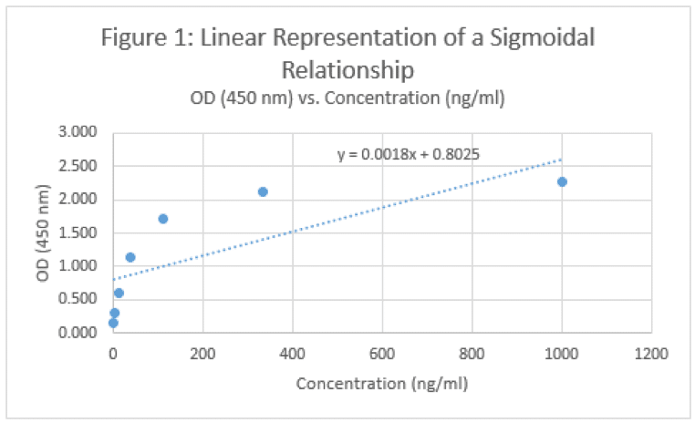Okay, well that doesn’t really look right.  And frankly, it doesn’t match what our eyes are telling us.  If we have a concentration of 1200 ng/mL, will the OD value be 3?  What about a concentration of 5000 ng/mL?  Will the OD be….6?  Will a concentration of 10,000 ng/mL melt the plate and burn holes in our eyes because it’s so bright? Of course not.  The data looks like it’s approaching a horizontal asymptote – a value that the curve will not pass.  So not matter how high your concentration goes, you’ll never get past 2.5 or so.  Similarly, this curve would seem to suggest that you can generate an OD value of ~0.5 if you have a negative concentration.  I’m no physicist, but that seems wrong too.  So, what’s another option?

The 4 Parameter Logistic Curve

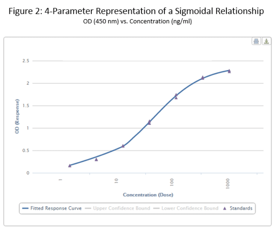
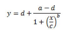
Finally, we come to the whole point of this article – the 4 Parameter Logistic Curve.  I will refer to this via its slang term – the S-curve.  The data below is the same that I used to generate the linear curve in Figure 1, but with a different format equation used to fit the data. Now, that’s more like it, right?  This curve very clearly shows both horizontal asymptotes – verifying what our eyes are seeing – and also shows a nice, dose-dependent response as the standard concentration increases or decreases.  I’m sure you also noticed the a-d values listed below the figure in Table 2.  These are derived from the curve, and fit into the equation below, where ‘y’ is our OD and ‘x’ is the corresponding concentration: In this equation, ‘a’ and ‘d’ represent the minimum and maximum values, respectively, that can be obtained – our asymptotes.  ‘C’ represents the point of inflection – the midpoint of your curve, and ‘b’ represents the slope of the curve at ‘c’.  Given this equation, we can now back-calculate an unknown concentration of one of our samples.  Fortunately, most of your plate readers probably have an option to do this for you automatically.  If not, Microsoft Excel does not handle this type of curve well.  There are some free options on the web.  Both elisaanalysis.com/app and www.myassays.com have tools that enable you to copy and paste plate reader data into their web app, which spits out one of these curves.

Using the S-Curve

When using these curves, it helps to keep a few practical tips in mind.  Since this graph starts and ends with asymptotes, you don’t have to be a mathematician to deduce that interpreting data outside the range of your curve will likely yield inaccurate results. Further to that point, try to work in the more linear range of your standard curve in the middle of the ‘S’.  Generally speaking, unknown calculations are more accurate in the linear range of the curve.  Finally, keep in mind that you can dilute samples that fall outside of your standard curve range.  If you’re expecting a final concentration of 2000 ng/mL, dilute 3-5X, determine the OD, calculate the concentration based on your standard curve, and then multiply this value by 3-5, respective to the initial dilution. Hopefully these equations and explanations here give you a better feel for the 4-paramter curve and the variables that are contributing to the formation of the equation that gets spat out by your computer.  Or if you’ve never seen one of these before, I trust that you’ve now seen the truth and will join us over on this side of the force.