Excelling With Excel: Analytical Method Validation Using LOD and LOQ

What’s the Point?

When performing an un-established analytical method, one needs to statistically validate it. Failing to do so, you might end up with erroneous results and waste time and resources. Limit of detection (LOD) and limit of quantitation (LOQ) are the two crucial parameters used to validate analytical methods. This article will describe what LOD and LOQ are, their importance in method validation, and finally a quick method to calculate these values using Excel.

What Are LOD and LOQ?

LOD and LOQ mean exactly what these terms suggest. They are the minimum amount of compound (analyte) that can be reliably detected and quantified, respectively, using an analytical method/instrument. [1]

When measuring the concentration of an analyte, the analyte must produce a signal greater than the analytical noise, i.e., the signal obtained in the absence of analyte. [1] If the analyte concentration is too low, the analyte signal cannot be distinguished from analytical noise. For this reason, a limit is set for the detection of the analyte (LOD), which is higher than the signals that fall in the analytical noise zone. This ensures that the signal is indeed due the analyte, and not due the analytical noise.

The Importance of Computing LOD and LOQ

In Validating a New Analytical Method

New analytical techniques can have a lot of advantages over tried-and-true methods. For example, HPLTC can be more cost effective and sensitive than the more traditional HPLC. If the concentration of the analyte you plan to detect using a certain analytical method that you developed is below the LOD and/or LOQ, then the signal you detect cannot be trusted. To ensure that your data are accurate and reliable, it is important to compute the LOD and LOQ for any new analytical technique.

In Validating Established Analytical Methods

It is also wise to compute LOD and LOQ for an already established method. Although you might try your best to avoid incorporating manual errors, there is still a good chance of that happening. For instance, pipetting errors can lead to variations in response when performing serial dilutions to prepare a standard curve. Furthermore, the sensitivity of every analytical technique differs with the instrument. Therefore, the standard curve you have freshly plotted requires statistical validation to ensure the responses of your test samples are within the range of detection/quantitation.

Calculating the LOD and LOQ Using MS Excel

Among the methods used to validate analytical methods, such as serial dilutions, computing LOD and LOQ via a calibration curve in MS Excel is more accurate and reliable. The serial dilution method defines the LOD as the concentration of analyte that gives you a response 95% of the time across a dilution series. Although the dilution subsequent to the assumed LOD (say ‘x’) might not give a response 95% of the time, there is a chance that a concentration between the assumed LOD and ‘x’ might. Thus, in the case of the serial dilution method, there is no exact figure that you can accurately/statistically term as the LOD. However, it may be used to verify the LOD that has been determined via other methods. [2]

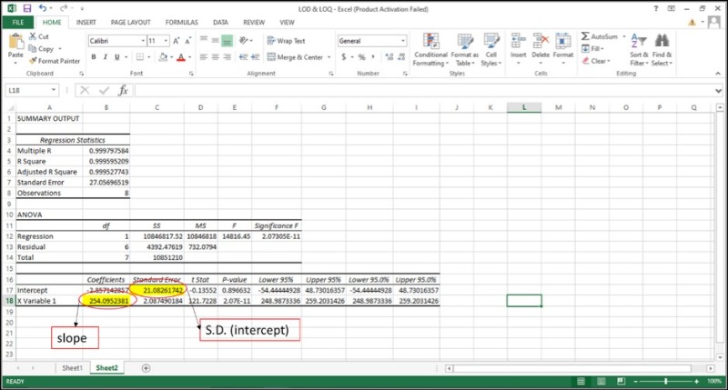
On the other hand, the calibration curve method using MS Excel is based on the standard deviation (SD) of response (\(\sigma\)) and slope (s) of the calibration curve, [3] thus making it more accurate. The SD (\(\sigma\)) can be calculated for the Y-intercept and used to calculate the LOD and LOQ for a standard curve using the regression function in MS Excel (I use version 2013; however, you can use any version and it’ll work just fine) as follows.

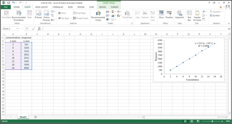
Step 1: Plot a Standard Curve

Construct a standard curve by plotting the concentration of analyte on the X-axis and the response on the Y-axis. Assuming the response is directly proportional to the analyte concentration, you should plot a linear curve.

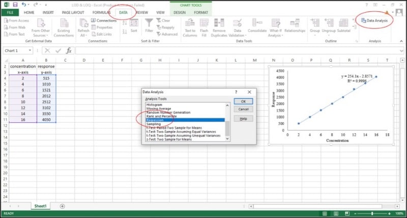
Step 2: Carry Out a Regression Analysis Using the Regression Function

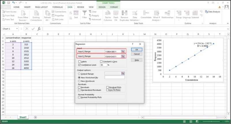
You can find the regression function under Data>Data Analysis>Regression. Under the regression function, select the data for the X and Y variables.

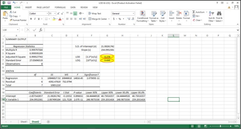
The regression function yields three outputs: regression statistics, ANOVA, and coefficients. Regression statistics tell you how well the regression equation fits the data, ANOVA gives you the level of variability within your regression model, and the coefficients (the most useful part) include the slope of the curve and the SD of the Y intercept. You now have a new Excel sheet with the data required to compute the LOD and LOQ.

Step 3: Use the \(\sigma\) and s values in the following formulae to compute the LOD and LOQ

LOD = [3.3*(\(\sigma\)/s)]

LOQ = [10*(\(\sigma\)/s)]

The coefficients 3.3 and 10 are called expansion factors and are obtained assuming a 95% confidence level. [4]

By computing the LOD and LOQ for your standard curve using this quick and simple method, you can rely on your data. Try this method to validate your analytical technique and let us know in the comments if you have excelled with Excel.

References

1. Armbruster, D.A., Pry T. Limit of blank, limit of detection and limit of quantitation. Clin. Biochem. Rev. 29, Suppl 1 (2008).
2. Ripp, J., Analytical Detection Limit Guidance & Laboratory Guide for Determining Method Detection Limits, Wisconsin Department of Natural Resources, Laboratory Certification Program, 1996. https://books.google.co.in/books?id=7WtjHQAACAAJ.
3. Shrivastava, A., Gupta, V. Methods for the determination of limit of detection and limit of quantitation of the analytical methods. Chronicles Young Sci. 2, 1 (2011). doi:10.4103/2229-5186.79345.
4. Desimoni, E., Brunetti, B. About Estimating the Limit of Detection by the Signal to Noise Approach. Pharm. Anal. Acta. 6, 4 (2015). doi:10.4172/2153-2435.1000355.

Sandesh Marathe

Sandesh earned his Ph.D. in Biotechnology in 2020, from the Institute of Chemical Technology, Mumbai. He is currently a Postdoctoral Researcher at the University of Tennessee Health Science Center (UTHSC), Memphis, US. His research interests include immunology, pharmacognosy, food bioscience, and functional foods and he is passionate about scientific writing.

Share this article: