Brushing Up On Your Excel Skills: Part Two

Last time we brushed up on cell referencing and constructing formulae to use Excel for some basic and some slightly more advanced calculations. This time we’re going to move on to using some built-in Excel functions and go through how to apply all that we’ve done so far to a worked example that is relevant to the lab.

Get Calculating

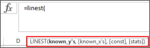
Now that we know how to correctly reference and fill in our calculations in Excel, it’s time to get started with some built-in functions. A nice feature of the functions in Excel is that once you select them and start typing, a small box will pop up underneath, which will give you the format you need to use with that particular function. For example, to use the function “Linest”, you need to enter groups for X and Y separated by commas, a constant followed by a comma, and decide if you want stats before closing the brackets. (We’ll go through all of those variables later so don’t worry about them just yet!)

If you get an error message or something doesn’t work out, a good place to start troubleshooting is by double-checking that your function is in the correct format and that you haven’t missed out a comma or bracket.

Excel has several hundred built-in functions for a variety of calculations, most of which I’m going to casually ignore; instead we’re going to focus in on four functions that can be handy around the lab.

Sum

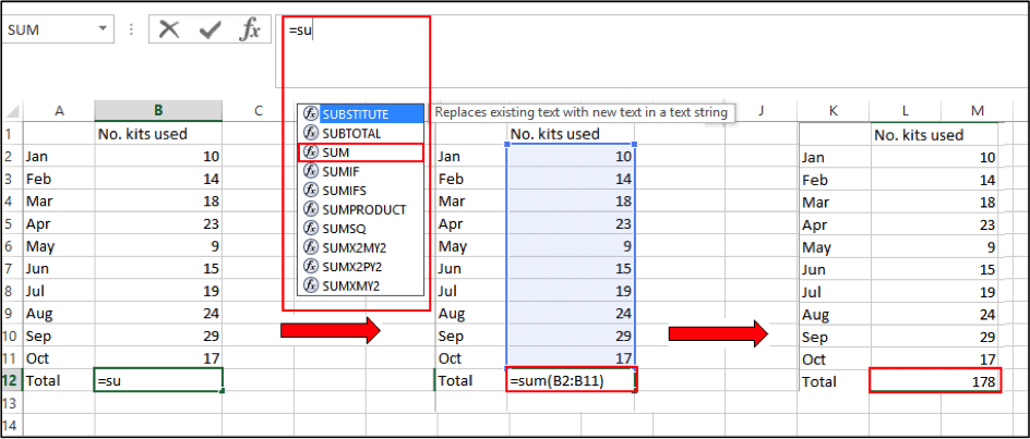
Sum, the most basic of the handy Excel functions, is just for adding the contents of cells together. You could easily type an addition calculation and skip the function altogether if you only have a small data set, but when you have multiple data points using a function can be considerably quicker.

1. In the cell you want your answer in, type =sum (Excel will start suggesting functions to use and you can either double click on these or manually type them in)
2. Open a set of round brackets
3. Select your data points by highlighting the boxes and close the brackets
4. Hit enter and let Excel do all the work!

Average

After sum, average is probably my most used Excel function, especially for things like analyzing values for samples I’ve run in triplicate. As with sum, simply;

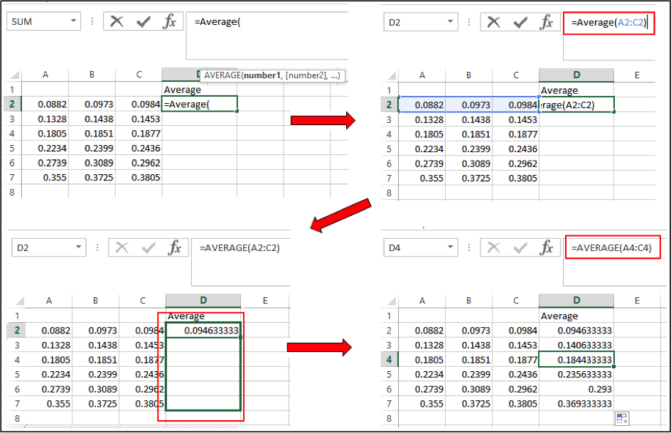
1. Select your box and type =average(
2. Highlight the appropriate boxes
3. For multiple samples, use the fill handle to copy the formula down the page
4. If you click on any of the other “average” boxes, you’ll see that the formula has changed from our original “average(A2:C2)” so that it is relative to the current row you’ve clicked on. This is because we used relative referencing and not absolute referencing.

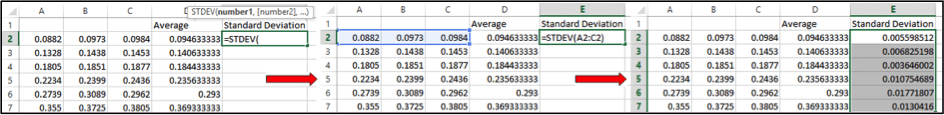
Stdev

The standard deviation (SD or ?) is often used to determine the variability of data, with a value close to 0 indicating that all data points are close to the mean; having the standard deviation beside your values can give you a good indication of the spread of your data. Standard deviation is calculated by taking the square root of the average of the squared differences of the values from the mean value…, which is confusing enough to write down, never mind calculate with a pen and paper! Instead;

1. In your cell enter =stdev(
2. Highlight your data set and close the bracket
3. Feel relieved that you didn’t have to do all those calculations yourself!

Linest

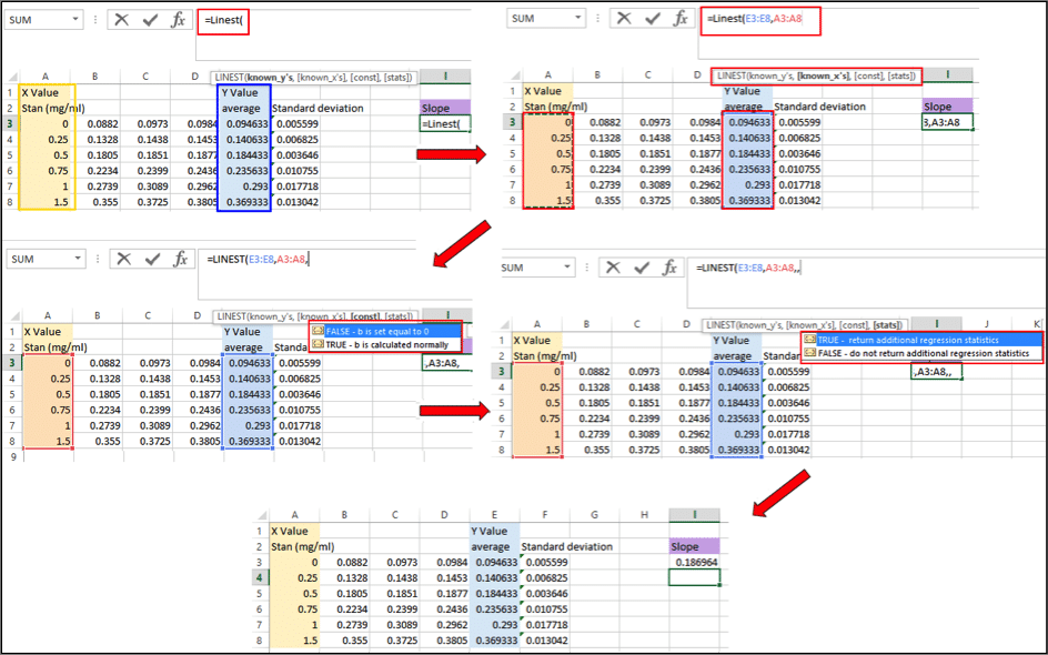
Moving on to slightly trickier territory, Linest is used to calculate the slope of a line, which can come in handy if you’re generating a standard curve. To use Linest, you must have a range of values for X and Y.

1. In your cell enter =Linest(
2. Highlight your Y values (in this case the average absorbance values in blue)
3. Insert a comma and highlight your X values (in this case the standards in yellow)
4. Insert a comma, the next value is for calculating where your line intercepts the axis, you can set this to 0, or you can leave it blank and allow Excel to determine the best point of intercept. To do this, just insert another comma and move on.
5. The final part of the function is about statistics. If you want values like your intercept, the standard error of intercept/slope/Y values, degrees of freedom, sum of square for regression etc. then type in “true”, or if you don’t need that sort of thing you can type “false” or leave it blank, just close the bracket and hit enter.

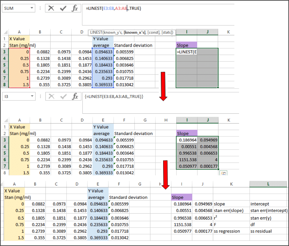
For you eager beavers looking for additional statistics;

6. Select the cell that contains your linest formula and drag the selection to include the cell to its right and down four rows
7. Go to the formula bar and click into the formula so that the X and Y values in the formula are highlighted
8. Hit Ctrl + Shift + Enter (or Cmd + Enter for Mac) and your stats will appear! Sadly they don’t appear with labels so you’ll need to keep a copy of the explainer list handy, shown below.

Practical example

Now that you can sum, average and linest with the best of them, let’s try putting everything together into a worked example – calculating the concentration of an unknown protein from a standard curve.

Start with your raw absorbance values:

Take the average for each standard:

The warning icon will appear because we haven’t included every number in the row – that’s because we don’t want to average the value of our standard so it’s OK to ignore this!

Using absolute referencing, subtract the blank value from your other standards.

Now have a quick look at your standard deviation to make sure your values are not too varied!

To plot your X and Y values:

1. Highlight your standard values (X) and your average absorbance value (Y).
2. Go to the “Insert” tab and insert and XY scatter plot.

3. Add a trendline by selecting one of the data point and right clicking.

Now that you have a graph, you can add in the equation of the line

4. Right click on your trendline and select “Format trendline”

5. Scroll through your trendline options and click “Display Equation on chart”

Now you can calculate your slope and intercept using Linest.

Bring in your unknown values.

Repeat the analysis you did for your standard samples; average, subtract blank, check standard deviation.

Now to calculate your value from the standard curve, remember that we have absorbance values (Y value) and we have a line with equation y=mx+c, manipulation of which will give us x=(y – c)/m

1. Select the cell and enter =
2. Using relative referencing for your sample (so that we get values for all samples) and absolute referencing for the slope and intercept (so that these remain constant) enter the formula =(F11-$K$2)/$J$2

Now all you need to do is correct for any dilutions you may have made and that’s you done!

That’s it for part two but check back with us soon for more Excel tips and tricks. Don’t forget to leave a comment if you have any hints of your own that you want to share!

*All screenshots are taken from Microsoft Excel 2013 for windows.