So, you’ve slaved away in the lab for months and now you’re ready to create your first figure –whether it’s for a thesis or a journal – way to go you!
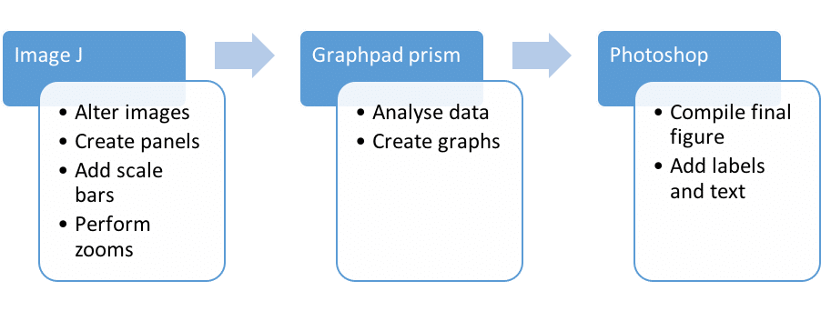
Now you could always use Word or PowerPoint to compile your first image, but don’t – ever do that! (And if you plan to then stop, read this article, and then go on to create amazing figures). Today’s professional software, like Photoshop or GIMP, enable you to create a highly polished images ready for publication. A word of caution though, be familiar with the journal requirements for figures before you start. The general workflow is as follows:
Step 1. Image Manipulation in Image J
It is always best to perform any manipulation of microscopy images using the appropriate software, for example image J. I will show you how to alter your image, add scale bars, perform zooms, and create panels ready for importing into Photoshop.
The first thing to do is to open your image for the first panel you create, for example, a microscopy image with a green and red channel. You may need to split your channels (Image > Colour > split channels).
Enjoying this article? Get hard-won lab wisdom like this delivered to your inbox 3x a week.

Join over 65,000 fellow researchers saving time, reducing stress, and seeing their experiments succeed. Unsubscribe anytime.
Next issue goes out tomorrow; don’t miss it.
Perform any relevant brightness and contrast enhancements, ensuring that the same settings are used for all images (Image > Adjust > Brightness and contrast) and then save a copy of the different channels as well as the merged image (Image > Colour > Merge channels).
Next, you will need to create a panel. To do this we will use the montage tool. Firstly, open your three images (green, red, and merged), and then create a stack from these images (Images > Stacks > Images to Stack). Next, use the montage tool (Image > Stacks > Montage) to create a panel of your images. Play around with the border width and scale factor, whilst adjusting the number of columns/rows as required. Save your panel at this point as a tiff file.

Now that you’ve got your first panel, you will also need a scale bar. Add one to the bottom right of your panel (Analyse > Tools > Scale bar). Be sure to make a note of the width. Save your panel, with the scale bar, as a tiff file.
At this point you may be happy to proceed, but let’s add a little clarity to our image by performing a zoom. To do this, draw a square around the region of interest (edit > Draw) and then copy this selection and paste the duplicate. You can now zoom as needed before saving.
Step 2. Creation of Graphs Using Graphpad Prism
With Graphpad prism, you get beautiful graphs. Alternatives, such as R are used by the more statistically savvy.

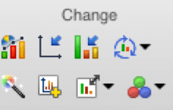
Open up prism and choose the most appropriate table type (column, XY etc.) and then plug in your data. Once you have entered your data, click to view your new graph (under the graphs folder).
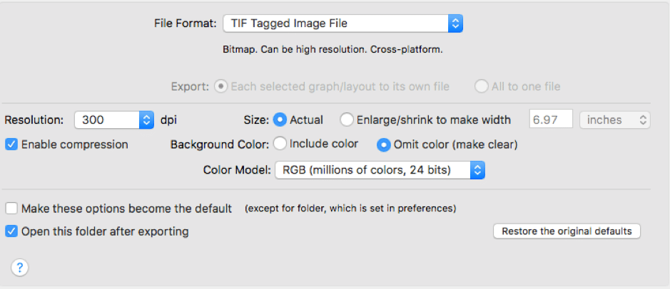
Go back to your table and use the analyse tool to perform statistical analysis of your data. Once finished, you are ready to export the graph. Go to File > Export.
Save your file as a TIF and set an appropriate resolution (600 dpi should usually suffice); leave the size as you wish, tick to enable compression, and select to omit colour (make clear) to remove the background white of your image. Leave your colour model as RGB and then save your file. These are generally useful settings but may change depending on preference or journal requirements.

Step 3. Final Figure Compiling in Photoshop
When you first open Photoshop, you are asked to set up the page. Refer to the journal requirements to do this, or set up a preferred page size – I use A5 as this fits brilliantly on an A4 page with margins. It is also best to keep your resolution high and then reduce it down to the journal requirements – 600dpi should suffice.
Just before we continue, the following table has some of the most useful shortcuts:
| Shortcut | Function |
| V | Move tool |
| U | Shape tool |
| T | Type tool |
| Ctrl + T | Transform |
| Ctrl + ; | Guides on/off |
| Ctrl + +/- | Zoom in/out |
| Ctrl + R | Rulers on/off |
You now have your blank canvas. Use the guides (click and drag down or across from the rulers to create a new guide line) to map out your planned layout.
Begin by dragging your saved panel image into Photoshop and then into your canvas using the move tool. Once here you can resize the panel to better fit your space using the transform tool (Crt + T) – Remember to keep the aspect ratio constant. You will need to press Enter or select the tick icon to confirm changes.
Now, all that is left is to add are the figure labels and any text. To do this, use the type tool (T) and add your text to the relevant places in your figure You can move the text using the move tool.
Save your completed figure as a Photoshop file (for later tweaking) and as a pdf file.
Step 3 (Alternative). Compiling Final Figures Using GIMP
GIMP is the free alternative to Photoshop and works in much the same way. When you first open GIMP, create a new page similar to how you would in Photoshop (File > New).
In GIMP, the shortcut keys are different but there is also a much larger and clearer layout in the toolbox window:
| Shortcut | Function |
| M | Move tool |
| Shift + T | Scale tool |
| T | Type tool |
Guides work exactly the same as they do in Photoshop, by dragging from a ruler and they can be turned on and off (View > Show guides).
Drag your saved panel images into GIMP and then place them in the appropriate place using the move tool. Once here you can resize the panel to better fit your space using the scale tool (Shift + T) – Remember to keep the aspect ratio constant by clicking on the chain link icon. Either drag the corners of the image or use the boxes provided. You will need to press scale to confirm your changes, or reset to undo your changes.
Add in labels using the type tool (T) just as you would in Photoshop, and use the move tool to re-position as necessary.
You now have a completed figure – Congratulations!
To learn more, there is an excellent series of YouTube videos on how to use Photoshop for scientists found here and a useful blog here.
There are also other Bitesize Bio articles that are definitely worth a read:
- Art of science figure creation
- Make illustrations and schematics with Illustrator
- Tips for better image processing in Photoshop
- Ethical Photoshopping
You made it to the end—nice work! If you’re the kind of scientist who likes figuring things out without wasting half a day on trial and error, you’ll love our newsletter. Get 3 quick reads a week, packed with hard-won lab wisdom. Join FREE here.


