
When optimizing qPCR, you might try trial and error to improve your assay’s performance. Tweak this, tweak that, and the assay works better, right? Sometimes you might get lucky but adjusting single assay components interdependent with others is hardly systematic. You can spend a lot of time and resources hoping that this time, you will get it just right. However, a systematic approach known as Design of Experiments (DoE), sets out to determine the cause and effect relationships between different factors (e.g. Mg++, dNTP and oligo concentration, etc.). Typically, numerous experiments are needed, but there is a simplified DoE method developed by Dr. Genichi Taguchi enabling quick trials with simple data analysis.
What Exactly Is Meant by Optimizing qPCR and Why Should You Care?
Before delving into the specifics of the Taguchi method, we need to define what is meant by the term optimization. Stated simply, it is the process where you determine the best set of conditions within a given context.
But what is maximum performance and how do you know when you’ve reached it? That depends on what you would like to accomplish with the assay and what constraints exist. For instance, is speed the priority or is sensitivity? Answers to this type of question will determine the context in which optimization experiments are performed. The optimal assay conditions then will differ in the context prioritizing speed versus the conditions prioritizing sensitivity.
Before optimizing qPCR, you must have prior knowledge and understanding about your qPCR system. For instance robust oligo design as outlined this Bitesize Bio article on qPCR primer design is an important consideration as is the choice of polymerase and cycling conditions as described in our article on faster PCR optimization.
Enjoying this article? Get hard-won lab wisdom like this delivered to your inbox 3x a week.

Join over 65,000 fellow researchers saving time, reducing stress, and seeing their experiments succeed. Unsubscribe anytime.
Next issue goes out tomorrow; don’t miss it.
What Is the Taguchi Method and Why Use It?
Now let’s get into how to apply the Taguchi method to optimizing qPCR. The Taguchi method relies upon the use of Orthogonal Arrays to provide a streamlined set of balanced experiments and a function known as the Signal-to-Noise Ratio (S/N). The signal, of course, is the PCR product yield.
Based on your prior knowledge of your qPCR, you can choose how many components to use in your experiments and how many levels. Let’s say that you will confine optimizing qPCR to determining the optimal concentrations of Mg++, dNTPs, oligos, SYBR green and polymerase and that you will test these at three different levels. You would set up your experiments according to a five-factor, four-level array as shown in Table 1. For ease, we will consider all four nucleotides as a single component and both primers as a single component. The nucleotides are present in equimolar concentrations, as are the forward and reverse primers.
Expt. | Mg++ | dNTPs] | Primers | Polymerase | SYBR |
1 | A | A | A | A | A |
2 | A | B | B | B | B |
3 | A | C | C | C | C |
4 | A | D | D | D | D |
5 | B | A | B | C | D |
6 | B | B | A | D | D |
7 | B | C | D | A | B |
8 | B | D | C | B | A |
9 | C | A | C | D | B |
10 | C | B | D | C | A |
11 | C | C | A | B | D |
12 | C | D | B | A | C |
13 | D | A | D | B | C |
14 | D | B | C | A | D |
15 | D | C | B | D | A |
16 | D | D | A | C | B |
What about the yield?
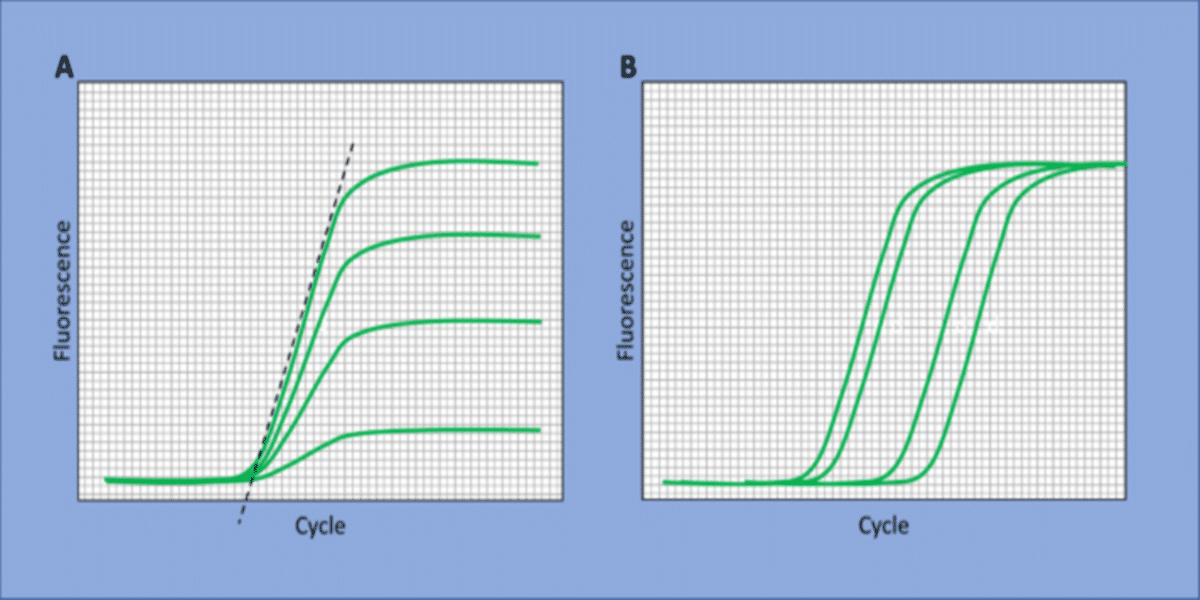
Here, yield can refer to the signal generated by the accumulation of PCR products and/or the efficiency of the reaction. Conditions generating more PCR product indicate a greater yield, as do conditions with greater reaction efficiency. These are not the only two examples, but they are both straightforward to determine. Let’s take a look at Figure 1, where both reaction efficiency (A) and product accumulation (B) are summarized.
Sticking with these two examples, we can define yield to select the S/N equation:
- Choose accumulation of PCR product: Reactions reaching a threshold cycle (Ct) earlier have accumulated more product in that amount of time than reactions reaching the Ct later. Since the smaller value for Ct is a greater yield of product, one selects the “smaller is better” equation 1.
OR
- Choose PCR efficiency: One calculates the amplification plot slopes. Steeper slopes reflect greater efficiency and thus a larger yield. Since steeper slopes are a larger numerical value than the shallower slopes of less efficient reactions, the “larger is better” equation 2 is selected.
This choice is a matter of preference and can be based on what is easier to calculate but should also be based on the understanding of your assay system. For example, if you are observing the Ct’s you’d like with the unoptimized assay, but see very shallow amplification plots, you might consider basing S/N on the slope of your amplification plots.
The Ct value or slope is the variable that would be entered for y in equation 1 or 2 respectively.
Equation 1
\( S/N = -10log_{10} \left[ \frac{\mathrm{1} }{\mathrm{n}} \sum\limits_{i=1}^{n} y^2 \right] \)
Equation 2
\( S/N = -10log_{10} \left[ \frac{\mathrm{1} }{\mathrm{n}} \sum\limits_{i=1}^{n} \frac{\mathrm{1} }{\mathrm{y^2}} \right] \)
Determine the Factors
As described above, factors refer to the reaction components or other assay parameters like thermal cycling temperatures and incubation times that will be put to the test and the selection is based on understanding your assay system. Per figure 1, this exercise will consider Mg++, dNTPs, primers, the polymerase and SYBR green as the five factors.
Choose Your Factor Levels
Again, you draw upon the prior knowledge of your assay system (see a trend?). Levels can be broad at first, say a range where levels are separated by 10-fold increments, and narrowed down in subsequent iterations, but should be set to a range that allows you to observe their effects on the reaction.
How orthogonal arrays are derived is beyond the scope of this article, but combinations of factors and levels are not unlimited. Fortunately for the biologist, numerous resources exist to for one to simply look them up! This from the University of York is one of them. After deciding on the range, choose a number of levels corresponding to an orthogonal array. This example uses four levels represented by the variable n in equations 1 and 2.
Analyzing Data
After running the 16 experiments outlined above, you would then calculate the S/N values and tabulate them as shown in figure 2A. This approach ultimately determines the single optimal concentration for each component by taking the following steps.
Calculate S/N values
- Summate the yields for each component at each level. As shown in figure 2A, if you were calculating the S/N for dNTPs at level B, you would use the yields from reactions where dNTPs were included at level B. In other words, you would plug in the yields from reactions 2, 6, 10 and 14 into either equation 1 or 2.
- Repeat this for each component at each level and you will have calculated a S/N value for A, B, C and D for each component.
Create the plots
- For each component, plot the S/N value against the corresponding component level (i.e. concentration). Note that each component is plotted on a separate graph. Figure 2B shows the plot for dNTPs and one would create separate plots for all five components.
- Fit the data points to a curve. This can be done using Microsoft Excel, but any graphing program that allows you to fit a curve to plotted datapoints could work. Curve fitting is essentially constructing a mathematical function represented by an equation. Figure 2B shows a cubic curve fit that would be represented by third-degree polynomial equation.
\( y=ax^3+bx^2+cx+d \)
Determine the maximum S/N values for each component
- Interpolate the maximum S/N value from each component’s fitted curve. Basically, you are interpolating the maximum value on the y-axis off the curve and this corresponds to the optimal concentration (x-axis) for that component. You can do this by eye, or more precisely by plugging values into the curve’s equation.
Just to reiterate, each component has its own curve, so you will go through these motions for each one and thereby derive the optimal component concentrations for the assay.
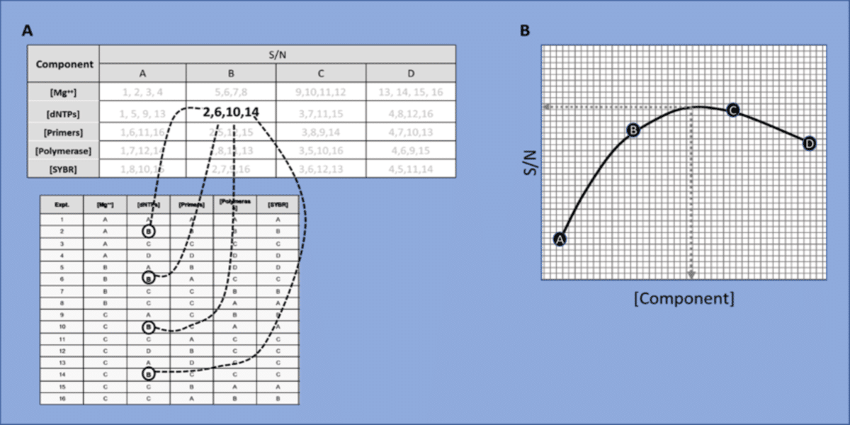
(A) Tabulation of S/N values for [dNTPs] at level B. Experiments 2, 6, 10 and 14 are where [dNTPs] were present at level B.
(B) plot of the S/N values derived at each level of the [component]. Interpolate the maximum S/N level from the fitted curve.
Confirming Results
Keep in mind, the optimal conditions are calculated and should be confirmed experimentally. You may consider testing the optimal conditions alongside some generic qPCR conditions to compare.
Additional Iterations and Duplex
If the conditions determined by the Taguchi method are indeed better than generic conditions, the next steps could include testing the performance of the optimized assay or even attempting additional iterations of the Taguchi method choosing levels clustered around those determined initially.
Finally, one limitation of the Taguchi method is that only one signal can be used for the S/N. If one is trying to optimize a duplex qPCR where each target is detected by a different probe, you could go through the motions of calculating the S/N using each probe’s signal as the basis. This would leave you with two sets of optimal conditions to test, where you would choose the best one. You might consider a multifactorial approach such as Response surface methodology if the Taguchi method did not help you achieve the desired assay performance.
Hopefully, you have come away with an understanding of the Taguchi method and can apply it to optimizing qPCR. This will save you from blindly testing out different assay conditions and help you systematically develop the best qPCR you can. We would love to hear what you think about this or other DoE strategies that have worked for you. Be sure to check out the additional resources and other Bitesize bio articles cited above!
Other Resources
Cobb BD, Clarkson JM. A simple procedure for optimizing the polymerase chain reaction (PCR) using modified Taguchi methods. Nucleic Acids Res. 1994;22(18):3801–3805. doi:10.1093/nar/22.18.3801
Thanakiatkrai, P, Welch, L. Using the Taguchi method for rapid quantitative PCR optimization with SYBR Green I. Int J Legal Med. 2012;126(1):161-165. doi:10.1007/s00414-011-0558-5
You made it to the end—nice work! If you’re the kind of scientist who likes figuring things out without wasting half a day on trial and error, you’ll love our newsletter. Get 3 quick reads a week, packed with hard-won lab wisdom. Join FREE here.


