SNPs or single nucleotide polymorphisms are on many scientist’s wish list in experimental studies of genomic DNA sequences. Methods to detect SNPs have evolved. Now with the availability of high throughput sequencing methods, also known as next generation sequencing (NGS), SNPs can be identified in the large amounts of DNA sequence that is generated. There is some research being done on SNPs in cell-free DNA (cfDNA). The identification of SNPs in such data relies on computational methods. They vary depending on whether you are interested in germline or somatic mutations, However, they generally align sequences back to a reference genome and make calls depending on the probability parameters you set.
However, NGS SNP calling or genotyping is no small feat. The obtained sequences often contain subtle yet complex errors involving uncertainties, biases, and pesky false positive results. This means that you have to get high quality NGS data, which requires careful library preparation (including DNA size selection) to obtain. Then again, you are not going to let that stop you from getting your hands on the high-quality data sets, are you? When all is said and done, here are the main steps to generate high-quality SNPs data set:
Call Out the Variants and Genotypes
In this first step, you will determine the positions where at least one of your samples differs from the reference sequence or otherwise known as “variant calling”. The next step, where you evaluate the individual alleles at all variant sites is known as “genotyping”. Large numbers of bioinformatic software can be used to help you find the variant within the NGS reads. For single-sample variant calling, you can use Atlas-SNP2, SLIDERII, and SOAPsnp. For genotyping or multi-sample variant calling, FreeBayes, GATK, QCALL, SAMtools, and SeqEM are good recommendations.
How you process your information depends on the type of sequence coverage you have. Sequencing coverage refers to the average number of times a single base is read during a sequencing experiment. Calculate it like this:
Put this article into practice
Choose a free resource to help you move forward
EBOOK
Gene Editing 101
DOWNLOAD
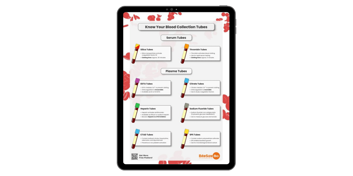
Blood Collection Tube Chart
Coverage = Read count x Read length / Target sequence size
For example, a 10x coverage means each base has been read by 10 sequences, while a 100x coverage means each base has been read by 100 sequences. The more frequently a base is sequenced, the higher the coverage of the reads, and the higher the reliability as well. Most publications require the level of coverage ranges from 10x to 50x depending on the research application. Certain cancer research might require 100x coverage to ensure the quality of the data.
With high coverage sequencing data, you could simply ignore the low-quality alleles and count only the high-quality alleles that you come across. On the other hand, if you are dealing with medium and low coverage sequencing data, you might want to use probabilistic or Bayesian methods to avoid undercalling of heterozygous genotypes. These take into consideration additional information before determining whether a given locus is heterozygous or homozygous. This includes information like read coverage, the error rate of the NGS platform, and alignment quality scores.
Increase Sensitivity with Joint Calling
I almost forgot to mention that you could also get your hands on data with high sensitivity and high specificity, by combining information from the initial alignment with the local short reads you have generated from scratch (de novo assembly). This method is called joint calling. Like almost any other in silico research, experimental design plays important roles in variant calling and genotyping. By using high coverage sequence data, you will get more specific variant calls and genotype estimations. However, due to limited research budgets…*looks at the wallet* *sigh*, forcing yourself to obtain high coverage will result in sequencing fewer samples. Thus, you will get a poor representation of a population’s true genetic variation.
On the other hand, using low coverage sequencing might provide a better picture of the population’s variation, but then again, it will have much higher uncertainties and errors. For that reason, you might want to use joint calling to reduce the systematic errors, sampling bias, and increase the strength of poorly supported variants. By doing this, you are getting the best of the both worlds. For this method to work, you need the appropriate software to perform the job, such as GATK’s HaplotypeCaller or Platypus. The results report in the variant calling format.
Filter out the error in SNPs
Next, you should remove the false positives from the initial genotype calling data set. By doing this, you will improve the specificity tremendously. First, there are two filtering strategies to choose from.
The first strategy is hard filtering. This strategy assumes that false positives often display unusual characteristics, for example:
- Low-quality scores in duplicated regions which lead to ambiguous alignment
- Poor alignment with the reference sequence caused by an incomplete reference sequence
- Strand bias (normally, genuine variants will have equal coverage on both forward and reverse strand. However, in this case, the variant is either only supported by the forward strand or reverse strand)
- A high number of variants clustering within certain region
In hard filtering, you will remove these problems by setting up the specific criteria for these variant characteristics and finally excluding variants which don’t fit the criteria. However, hard filtering is often knotty because of uneven coverage (human major histocompatibility complex or leukocyte antigen gene) and repetitive regions (telomeres or centromeres). This type of filtering takes place in GATK VariantFiltration and VCFtools.
The second strategy uses soft filtering which generates reliable results with high coverage data sets. The strategy itself also uses machine learning methods to tackle specificity issues at lower coverage. Then again, this strategy is not without flaws. A major downside to this strategy is the need for large data sets of high-quality variants from previous studies. Hence, it is currently limited to animal studies which already possess extensive and accessible variant databases. GATK VQRS software can help you with this strategy.
Double Check Your Variants Quality (again)
Prepare for trouble and make it double! I can’t stress enough the importance of double checking your variants quality throughout the process. Do so either by visual inspection or validating your experiment using independent technologies. For visual inspection, you can use software, such as IGV, GenomeView, and SAVANT. You should also assess the overall quality of the dataset using simple calculations.
First, the number of observed SNPs should be within the estimated range of the species’ diversity[1]. Next, the number of SNPs should correlate with the chromosome physical length [2]. Finally, the ratios of homozygous and heterozygous genotypes should not violate the Hardy-Weinberg law, which means every diploid individual carrying a SNP should exhibit an allele frequency of either 1.0 for a homozygous or 0.5 for a heterozygous individual at the SNP locus[1] [3]. That’s all for now! Got any questions or tips that I might have left out in this article? Feel free to comment below.
Further Reading
1. Pfeifer SP. (2017) From next-generation resequencing reads to a high-quality variant data set. Heredity 118: 111-114. doi:10.1038/hdy.2016.102.
2. Tsai HY, Robledo D, Lowe NR, Bekaert M, Taggart JB, Bron JE, and Houston RD (2016). Construction and annotation of a high density SNP linkage map of the atlantic salmon (Salmo salar) genome. G3 (Bethesda) 6(7): 2173–2179.
3. Nielsen R, Korneliussen T, Albrechtsen A, Li Y, Wang J (2012). SNP calling, genotype calling, and sample allele frequency estimation from new-generation sequencing data. PLoS One 7: e37558.
4. Nielsen R, Paul JS, Albrechtsen A, Song YS (2011). Genotype and SNP calling from next generation sequencing data. Nat Rev Genet. 12: 443–451.
You made it to the end—nice work! If you’re the kind of scientist who likes figuring things out without wasting half a day on trial and error, you’ll love our newsletter. Get 3 quick reads a week, packed with hard-won lab wisdom. Join FREE here.
Put this article into practice
Choose a free resource to help you move forward
EBOOK
Gene Editing 101
DOWNLOAD
Blood Collection Tube Chart


