Five Simple Steps For a Successful MTS Assay!

The MTS cell viability assay is one of the most important yet often daunting assays to perform for researchers in cancer biology, immunology, drug delivery pharmacy, etc. This chromogenic assay is extremely dependable for assessing the effects of a drug on different cell lines. However, it is only an easy assay to master if you perform it carefully, paying attention to every step in detail. (Well, I learnt it the hard way and had to struggle with it for one whole month to master it! Haha!)

But trust me, once you follow all the steps to the book then I guarantee fantastic results! Below are five steps that I have found to be the most crucial (since I work mainly on cancer therapeutics this article focuses on cancer and immune cell lines of both mouse and human origin).

STEP ONE: Always keep an eye on the count!

One of the most common mistakes that everyone makes is ignoring the number of cells plated in each well. Remember: the number is not constant across cell lines. Different cells grow at different rates, for example, aggressive cancer cell lines like the B16 F10 mouse melanoma cells grow very quickly and have a doubling time of a few hours, whereas immune cells, like dendritic cells, take a relatively long time to grow and may even take a day to double.

To make things easy, I have optimized the cell number across every cell line and tabulated it as follows:

STEP TWO: Pay attention to the time at which you add the drug

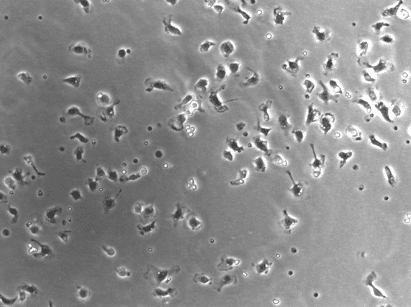
Another aspect of the assay which is commonly ignored is the time at which the drug treatment is added. The assay is based on the metabolism of cells so its success and failure depends mainly on the time of treatment. Ideally you want to start treatment when the cells are in their growth phase and not when they have reached complete confluence. If the cells are too confluent, you can miss significant effects of drug treatment when using lower concentrations of drug.

 

STEP THREE: Store and use reagents properly

Most of the reagents used in the assay are sensitive to light and need to be protected from it. This includes the MTS reagent, phenazine methyl sulphate (PMS) or phenazine ethyl sulphate (PES).

You should also use media that is devoid of phenol red as phenol red can interfere with the absorbance reading. Cell media should also be stored away from light as it contains HEPES which releases free radicals when exposed to light. The details of the preparation can be found in the manual from Promega.

STEP FOUR: Time becomes THE factor again!

Yes you hear me right, after you add the MTS reagent following drug treatment, you have to read the absorbance using a plate reader at a wavelength of 490nm. The tricky part here is to read the plate at the correct time. Too early, and the cells have no time to take up the PMS (electron carrier); too late, and the wells become over saturated and every well looks the same (dark brown).

Therefore, I also optimized the time at which a reading should be taken post MTS addition:

STEP FIVE: The math is important too!

All that starts well has to end well; your experiment becomes a success only after you learn to process and present your data in a precise manner. The following steps are rationally designed in order to get accurate cell viability values post-treatment with a drug/inhibitor. The efficacy of the drug/inhibitor is seen in terms of its IC50 value. The lower the value, more potent it is.

Calculations involved:

• Subtract the absorbance of the blank wells from all the wells.
• Divide the absorbance of the wells which have the cells treated with the drug/inhibitor by the average of the absorbances emitted from the cells in the control wells. This gives you the ratio of the number of dead cell to the number of living cells.
• Multiply the ratio by 100 to give you the viability in %.

Graphing:

Use the cell viability values to graph the data. I like to use Graphpad Prism 6 because it has built-in dose response functions.

After entering the software you can use one of the in-built functions of the software that is Dose response where the x- axis is log (dosage).

 

• Plot the data as a dose response curve in which the x-axis is the log of the dosage
• Generally it is better to have triplicates of the viabilities to reduce the error
• Analyze the data using non-linear regression and with three parameters (triplicates) to generate the IC50 values
• The final data should look something like this (or much better than this!):